You can download and run the notebook locally or run it with Google Colaboratory:
![]()
Best Practices for training CEBRA models#
We show you how to get started with CEBRA:
Define a CEBRA-Time model (we strongly recommend starting with this).
Load data.
Perform train/validation splits.
Train the model.
Check the loss functions.
Save the model & reload.
Transform the model on train/val.
Evaluate Goodness of Fit.
Visualize the embeddings.
Compute and display the Consistency between runs (n=10).
Run a (small) grid search for model parameters.
Once you have a good CEBRA-Time model, then you can do hypothesis testing with CEBRA-Behavior:
Define a CEBRA-Behavior model.
as above, train, check, evaluate, transform, and test consistency.
Run controls with shuffled data - which is critical for label-guided embeddings.
[ ]:
!pip install --pre 'cebra[datasets,integrations]'
[ ]:
import sys
import numpy as np
import matplotlib.pyplot as plt
import cebra.datasets
from cebra import CEBRA

#for model saving:
import os
import tempfile
from pathlib import Path
1. Set up a CEBRA model#
Items to consider#
We recommend starting with an unsupervised approach (CEBRA-Time).
We recommend starting with defaults, perform the sanity checks we suggest below, then performing a grid search if needed.
We are going to largely follow the recommendations from our Quick Start scikit-learn API
[ ]:
# 1. Define a CEBRA model
cebra_model = CEBRA(
    model_architecture="offset10-model", #consider: "offset10-model-mse" if Euclidean
    batch_size=512,
    learning_rate=3e-4,
    temperature=1.12,
    max_iterations=5000, #we will sweep later; start with default
    conditional='time', #for supervised, put 'time_delta', or 'delta'
    output_dimension=3,
    distance='cosine', #consider 'euclidean'; if you set this, output_dimension min=2
    device="cuda_if_available",
    verbose=True,
    time_offsets=10
)
2. Load the data#
(or adapt and use your data)
We are going to use demo data. The data will be automatically downloaded into a
/datafolder.
[ ]:
#2. example data
%mkdir data
hippocampus_pos = cebra.datasets.init('rat-hippocampus-single-achilles')
100%|██████████| 10.0M/10.0M [00:01<00:00, 9.52MB/s]
Download complete. Dataset saved in 'data/rat_hippocampus/achilles.jl'
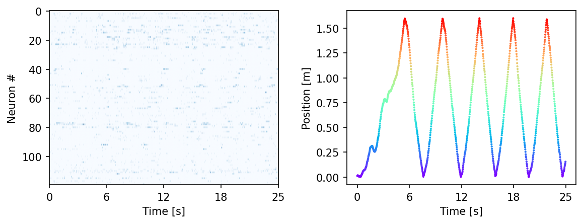
Visualize the data#
[ ]:
fig = plt.figure(figsize=(9,3), dpi=150)
plt.subplots_adjust(wspace = 0.3)
ax = plt.subplot(121)
ax.imshow(hippocampus_pos.neural.numpy()[:1000].T, aspect = 'auto', cmap = 'Blues')
plt.ylabel('Neuron #')
plt.xlabel('Time [s]')
plt.xticks(np.linspace(0, 1000, 5), np.linspace(0, 0.025*1000, 5, dtype = int))

ax2 = plt.subplot(122)
ax2.scatter(np.arange(1000), hippocampus_pos.continuous_index[:1000, 0],
            c=hippocampus_pos.continuous_index[:1000, 0], cmap='rainbow', s=1)

plt.ylabel('Position [m]')
plt.xlabel('Time [s]')
plt.xticks(np.linspace(0, 1000, 5), np.linspace(0, 0.025*1000, 5, dtype = int))
plt.show()
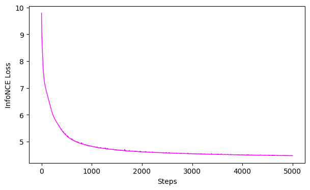
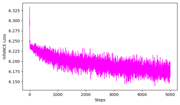
Quick test: Train CEBRA-Time on the full data (not train/validation yet)…#
This is a rapid quick start, just training without labels on the full dataset on the model we set up above! Here, we should already see a nice structured embedding.
Note, the colors here are post-hoc applied; positional information was not used to train the model.
[ ]:
# fit
cebra_time_full_model = cebra_model.fit(hippocampus_pos.neural)
# transform
cebra_time_full = cebra_model.transform(hippocampus_pos.neural)
# GoF
gof_full = cebra.sklearn.metrics.goodness_of_fit_score(cebra_time_full_model, hippocampus_pos.neural)
print(" GoF in bits - full:", gof_full)
# plot embedding
fig = cebra.integrations.plotly.plot_embedding_interactive(cebra_time_full, embedding_labels=hippocampus_pos.continuous_index[:,0], title = "CEBRA-Time (full)", markersize=3, cmap = "rainbow")
fig.show()
# plot the loss curve
ax = cebra.plot_loss(cebra_time_full_model)
pos: -0.8468 neg:  6.3701 total:  5.5233 temperature:  1.1200: 100%|██████████| 5000/5000 [00:46<00:00, 106.47it/s]
100%|██████████| 500/500 [00:01<00:00, 282.00it/s]
GoF in bits - full: 1.0338272469913845
<Figure size 500x500 with 0 Axes>
3. Create a Train/Validation Split#
now that we know we get something decent (see structure, proper loss curve), we can properly test parameters.
[ ]:
# 3. Split data and labels (labels we use later!)
from sklearn.model_selection import train_test_split
split_idx = int(0.8 * len(hippocampus_pos.neural)) #suggest: 5%-20% depending on your dataset size

train_data = hippocampus_pos.neural[:split_idx]
valid_data = hippocampus_pos.neural[split_idx:]

train_continuous_label = hippocampus_pos.continuous_index.numpy()[:split_idx]
valid_continuous_label = hippocampus_pos.continuous_index.numpy()[split_idx:]
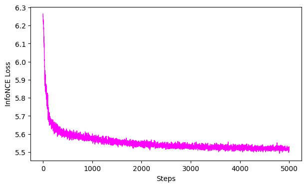
4. Fit the train split model#
[ ]:
cebra_train_model = cebra_model.fit(train_data)#, train_continuous_label)
pos: -0.8467 neg: 6.3683 total: 5.5216 temperature: 1.1200: 100%|██████████| 5000/5000 [00:46<00:00, 106.60it/s]
5. Save the model [optional]#
[ ]:
tmp_file = Path(tempfile.gettempdir(), 'cebra.pt')
cebra_train_model.save(tmp_file)
#reload
cebra_train_model = cebra.CEBRA.load(tmp_file)
6. Compute (transform) the embedding on train and validation data#
[ ]:
train_embedding = cebra_train_model.transform(train_data)
valid_embedding = cebra_train_model.transform(valid_data)
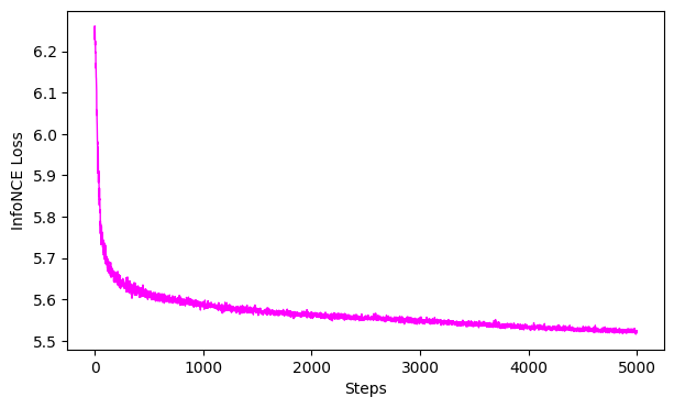
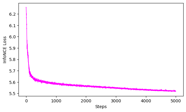
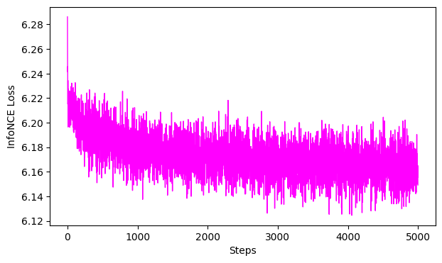
7. Evaluate the Model#
Plot the loss curve
We can also look at the Goodness of Fit this in bits vs. the infoNCE loss. See more info here
ProTip: 0 bits would be a perfectly collapsed embedding. Note, using GoF on the validation set is prone to low data regime issues, hence one should use the train loss to evaluate the model.
[ ]:
gof_train = cebra.sklearn.metrics.goodness_of_fit_score(cebra_train_model, train_data)
print(" GoF bits - train:", gof_train)

# plot the loss curve
ax = cebra.plot_loss(cebra_train_model)
100%|██████████| 500/500 [00:01<00:00, 287.01it/s]
GoF bits - train: 1.03642225468614
Visualize the embeddings#
train, then validation
[ ]:
import cebra.integrations.plotly
#train
fig = cebra.integrations.plotly.plot_embedding_interactive(train_embedding,
                                                           embedding_labels=train_continuous_label[:,0],
                                                           title = "CEBRA-Time Train",
                                                           markersize=3,
                                                           cmap = "rainbow")
fig.show()

#validation
fig = cebra.integrations.plotly.plot_embedding_interactive(valid_embedding,
                                                           embedding_labels=valid_continuous_label[:,0],
                                                           title = "CEBRA-Time-validation",
                                                           markersize=3,
                                                           cmap = "rainbow")
fig.show()
<Figure size 500x500 with 0 Axes>
<Figure size 500x500 with 0 Axes>
Next sanity/validation step: Consistency#
What did we check above?
do we see structure in our embedding? (if not, something is off!)
is the GoF reasonable? (infoNCE low, bits high)
Is the loss converging without overfitting (no sudden drop after many interations?)
IF 1-3 are not satisfactory, skip to the Grid Search Below!
Beyond these being met, we need to check the consistency across runs! In addition to the above checks, once we have a converging model that produces consistent embeddings, then we know we have good model parameters! 🚀
[ ]:
### Now we are going to run our train/val. 5-10 times to be sure they are consistent!

X = 5  # Number of training runs
model_paths = []  # Store file paths

for i in range(X):
    print(f"Training 🦓CEBRA model {i+1}/{X}")

    # Train and save model
    cebra_train_model = cebra_model.fit(train_data)
    tmp_file = Path(tempfile.gettempdir(), f'cebra_{i}.pt')
    cebra_train_model.save(tmp_file)
    model_paths.append(tmp_file)

### Reload models and transform data
train_embeddings = []
valid_embeddings = []

for tmp_file in model_paths:
    cebra_train_model = cebra.CEBRA.load(tmp_file)
    train_embeddings.append(cebra_train_model.transform(train_data))
    valid_embeddings.append(cebra_train_model.transform(valid_data))
Training 🦓CEBRA model 1/5
pos: -0.8449 neg: 6.3694 total: 5.5245 temperature: 1.1200: 100%|██████████| 5000/5000 [00:46<00:00, 106.60it/s]
Training 🦓CEBRA model 2/5
pos: -0.8525 neg: 6.3717 total: 5.5193 temperature: 1.1200: 100%|██████████| 5000/5000 [00:47<00:00, 106.28it/s]
Training 🦓CEBRA model 3/5
pos: -0.8493 neg: 6.3685 total: 5.5192 temperature: 1.1200: 100%|██████████| 5000/5000 [00:46<00:00, 106.51it/s]
Training 🦓CEBRA model 4/5
pos: -0.8403 neg: 6.3713 total: 5.5310 temperature: 1.1200: 100%|██████████| 5000/5000 [00:47<00:00, 106.16it/s]
Training 🦓CEBRA model 5/5
pos: -0.8511 neg: 6.3738 total: 5.5227 temperature: 1.1200: 100%|██████████| 5000/5000 [00:46<00:00, 106.62it/s]
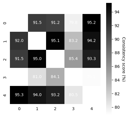
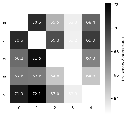
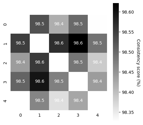
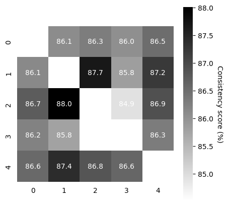
Compute Consistency Across Runs#
Now that we have 5-10 model runs, we can compute the consistency between runs.
TRAIN: This should be high (in the 90’s on the train embeddings)! If not, in this demo, we simply suggest training slightly longer.
VALID: Depending on how large your validation data are, this also should be as high.
In our demo data, the cebra-time on rat 1 with 20% held out is in the 70’s for 5K iterations, which is acceptable. One could consider training for longer (~8-9K).
[ ]:
scores, pairs, ids_runs = cebra.sklearn.metrics.consistency_score(
    embeddings=train_embeddings,
    between="runs"
)

cebra.plot_consistency(scores, pairs, ids_runs)
<Axes: >
[ ]:
scores, pairs, ids_runs = cebra.sklearn.metrics.consistency_score(
    embeddings=valid_embeddings,
    between="runs"
)

cebra.plot_consistency(scores, pairs, ids_runs)
<Axes: >
What if I don’t have good parameters? Let’s do a grid search…#
[ ]:
#%mkdir saved_models

params_grid = dict(
    output_dimension = [3, 6],
    time_offsets = [5, 10],
    model_architecture='offset10-model',
    temperature_mode='constant',
    temperature=[0.1, 1.0],
    max_iterations=[5000],
    device='cuda_if_available',
    num_hidden_units = [32, 64],
    verbose = True)

datasets = {"dataset1": train_data}
# run the grid search
grid_search = cebra.grid_search.GridSearch()
grid_search.fit_models(datasets, params=params_grid, models_dir="saved_models")
/usr/local/lib/python3.11/dist-packages/cebra/__init__.py:118: UserWarning:

Your code triggered a lazy import of cebra.grid_search. While this will (likely) work, it is recommended to add an explicit import statement to you code instead. To disable this warning, you can run ``cebra.allow_lazy_imports()``.

pos: -9.8901 neg:  16.0103 total:  6.1202 temperature:  0.1000: 100%|██████████| 5000/5000 [00:37<00:00, 133.92it/s]
pos: -9.7216 neg:  16.0270 total:  6.3053 temperature:  0.1000: 100%|██████████| 5000/5000 [00:36<00:00, 136.32it/s]
pos: -0.9863 neg:  9.1650 total:  8.1787 temperature:  1.0000: 100%|██████████| 5000/5000 [00:36<00:00, 135.48it/s]
pos: -0.9681 neg:  9.1653 total:  8.1972 temperature:  1.0000: 100%|██████████| 5000/5000 [00:36<00:00, 136.02it/s]
pos: -9.5956 neg:  14.2764 total:  4.6809 temperature:  0.1000: 100%|██████████| 5000/5000 [00:36<00:00, 137.69it/s]
pos: -9.5427 neg:  14.2884 total:  4.7457 temperature:  0.1000: 100%|██████████| 5000/5000 [00:36<00:00, 136.66it/s]
pos: -0.9697 neg:  9.1099 total:  8.1403 temperature:  1.0000: 100%|██████████| 5000/5000 [00:36<00:00, 137.57it/s]
pos: -0.9640 neg:  9.1295 total:  8.1654 temperature:  1.0000: 100%|██████████| 5000/5000 [00:36<00:00, 137.48it/s]
pos: -9.9187 neg:  16.0083 total:  6.0896 temperature:  0.1000: 100%|██████████| 5000/5000 [00:37<00:00, 134.27it/s]
pos: -9.7743 neg:  16.0204 total:  6.2462 temperature:  0.1000: 100%|██████████| 5000/5000 [00:37<00:00, 133.42it/s]
pos: -0.9860 neg:  9.1651 total:  8.1792 temperature:  1.0000: 100%|██████████| 5000/5000 [00:37<00:00, 134.29it/s]
pos: -0.9730 neg:  9.1657 total:  8.1927 temperature:  1.0000: 100%|██████████| 5000/5000 [00:37<00:00, 134.07it/s]
pos: -9.7831 neg:  14.2553 total:  4.4721 temperature:  0.1000: 100%|██████████| 5000/5000 [00:36<00:00, 135.51it/s]
pos: -9.7688 neg:  14.2423 total:  4.4735 temperature:  0.1000: 100%|██████████| 5000/5000 [00:36<00:00, 135.27it/s]
pos: -0.9752 neg:  9.0934 total:  8.1182 temperature:  1.0000: 100%|██████████| 5000/5000 [00:36<00:00, 135.69it/s]
pos: -0.9746 neg:  9.1277 total:  8.1531 temperature:  1.0000: 100%|██████████| 5000/5000 [00:36<00:00, 135.31it/s]
<cebra.grid_search.GridSearch at 0x7b54c2df3e10>
[ ]:
# Get the results
df_results = grid_search.get_df_results(models_dir="saved_models")

# Get the best model for a given dataset
best_model, best_model_name = grid_search.get_best_model(dataset_name="dataset1", models_dir="saved_models")
print("The best model is:", best_model_name)
The best model is: num_hidden_units_64_output_dimension_6_temperature_0.1_time_offsets_5_dataset1
[ ]:
#load the top model ✨
model_path = Path("/content/saved_models") / f"{best_model_name}.pt"
top_model = cebra.CEBRA.load(model_path)

#transform:
top_train_embedding = top_model.transform(train_data)
top_valid_embedding = top_model.transform(valid_data)

# plot the loss curve
ax = cebra.plot_loss(top_model)


# plot embeddings
fig = cebra.integrations.plotly.plot_embedding_interactive(top_train_embedding,
                                                           embedding_labels=train_continuous_label[:,0],
                                                           title = "top model - train",
                                                           markersize=3,
                                                           cmap = "rainbow")
fig.show()

fig = cebra.integrations.plotly.plot_embedding_interactive(top_valid_embedding,
                                                           embedding_labels=valid_continuous_label[:,0],
                                                           title = "top model - validation",
                                                           markersize=3,
                                                           cmap = "rainbow")
fig.show()
<Figure size 500x500 with 0 Axes>
<Figure size 500x500 with 0 Axes>
CEBRA-Behavior: using auxiliary labels for hypothesis testing#
Now that you have good parameters for a self-supervised embedding, the next goal is to understand which behavioral labels are contributing to the model fit.
Thus, we will use labels, such as position, for testing.
⚠️ We test model consistency on train/validation splits.
Then, we perform shuffle controls.
[ ]:
# Define the model
# consider changing based on search/results above
cebra_behavior_model = CEBRA(model_architecture='offset10-model',
                        batch_size=512,
                        learning_rate=3e-4,
                        temperature=1,
                        output_dimension=3,
                        max_iterations=5000,
                        distance='cosine',
                        conditional='time_delta', #using labels
                        device='cuda_if_available',
                        verbose=True,
                        time_offsets=10)
[ ]:
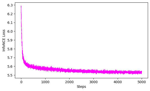
# fit
cebra_behavior_full_model = cebra_behavior_model.fit(hippocampus_pos.neural,hippocampus_pos.continuous_index.numpy())
# transform
cebra_behavior_full = cebra_behavior_full_model.transform(hippocampus_pos.neural)
# GoF
gof_full = cebra.sklearn.metrics.goodness_of_fit_score(cebra_behavior_full_model, hippocampus_pos.neural,hippocampus_pos.continuous_index.numpy())
print(" GoF in bits - full:", gof_full)
# plot embedding
fig = cebra.integrations.plotly.plot_embedding_interactive(cebra_behavior_full, embedding_labels=hippocampus_pos.continuous_index[:,0], title = "CEBRA-Behavior (full)", markersize=3, cmap = "rainbow")
fig.show()
# plot the loss curve
ax = cebra.plot_loss(cebra_behavior_full_model)
pos: -0.9066 neg:  6.4136 total:  5.5069 temperature:  1.0000: 100%|██████████| 5000/5000 [00:48<00:00, 104.04it/s]
100%|██████████| 500/500 [00:01<00:00, 264.61it/s]
GoF in bits - full: 1.037317863283606
<Figure size 500x500 with 0 Axes>
Test model consistency#
run train/valid.
[ ]:
# Now we are going to run our train/val. 5-10 times to be sure they are consistent!

X = 5  # Number of training runs
model_paths = []  # Store file paths

for i in range(X):
    print(f"Training 🦓CEBRA model {i+1}/{X}")

    # Train and save model
    cebra_behavior_train_model = cebra_behavior_model.fit(train_data,train_continuous_label)
    tmp_file2 = Path(tempfile.gettempdir(), f'cebra_behavior_{i}.pt')
    cebra_behavior_train_model.save(tmp_file2)
    model_paths.append(tmp_file2)

# Reload models and transform data
train_behavior_embeddings = []
valid_behavior_embeddings = []

for tmp_file2 in model_paths:
    cebra_behavior_train_model = cebra.CEBRA.load(tmp_file2)
    train_behavior_embeddings.append(cebra_behavior_train_model.transform(train_data))
    valid_behavior_embeddings.append(cebra_behavior_train_model.transform(valid_data))
Training 🦓CEBRA model 1/5
pos: -0.8775 neg: 6.4178 total: 5.5403 temperature: 1.0000: 100%|██████████| 5000/5000 [00:48<00:00, 103.75it/s]
Training 🦓CEBRA model 2/5
pos: -0.8972 neg: 6.4214 total: 5.5242 temperature: 1.0000: 100%|██████████| 5000/5000 [00:48<00:00, 103.15it/s]
Training 🦓CEBRA model 3/5
pos: -0.8953 neg: 6.4184 total: 5.5231 temperature: 1.0000: 100%|██████████| 5000/5000 [00:48<00:00, 103.77it/s]
Training 🦓CEBRA model 4/5
pos: -0.8951 neg: 6.4196 total: 5.5246 temperature: 1.0000: 100%|██████████| 5000/5000 [00:48<00:00, 103.78it/s]
Training 🦓CEBRA model 5/5
pos: -0.8806 neg: 6.4167 total: 5.5360 temperature: 1.0000: 100%|██████████| 5000/5000 [00:48<00:00, 103.98it/s]
[ ]:
gof_train = cebra.sklearn.metrics.goodness_of_fit_score(cebra_behavior_train_model, train_data, train_continuous_label)
print(" GoF bits - train:", gof_train)

ax = cebra.plot_loss(cebra_behavior_train_model)
100%|██████████| 500/500 [00:01<00:00, 271.85it/s]
GoF bits - train: 1.0219604963645763
[ ]:
#train
scores, pairs, ids_runs = cebra.sklearn.metrics.consistency_score(
    embeddings=train_behavior_embeddings,
    between="runs"
)

cebra.plot_consistency(scores, pairs, ids_runs)

#validation
scores, pairs, ids_runs = cebra.sklearn.metrics.consistency_score(
    embeddings=valid_behavior_embeddings,
    between="runs"
)

cebra.plot_consistency(scores, pairs, ids_runs)
<Axes: >
The next item to do when using labels is to perform shuffle controls#
Why do we do this? It is entirely expected that the distribution of the labels shape the embedding (see Proposition 7, Supplementary Note 2). In Figure 2c we therefore show shuffle controls should be performed, and demonstrate that if labels are shuffled, it is not possible to fit them.
In our paper we shuffle the labels across time. When the
time_deltastrategy for positive sampling is used, this changes the distribution of the positive samples. We do this kind of control to show that fitting a model on nonsensical label structure (in a real experiment, this would be a behavior time series without connection to the neural data) is not possible (assuming a sufficiently large dataset).
Another approach is to shuffle the neural data. However, if the model has sufficient capacity (is large), the data is limited, and one trains too long, it can fit a “lookup table” from input data to the output embedding to match the label distribution (because this is intact and still has structure). Thus, this can be useful to be sure you are not overparameterizing or training too long!
If you shuffle the neural data, the question is whether the label structure can be forced on a latent representation of the shuffled data. This will be possible as long as the model has enough capacity to fit a lookup table, where for each timepoint the embedding is arranged to fit the behavior.
Label-Shuffle Control#
[ ]:
# Label Shuffle control model:
cebra_shuffled_model = CEBRA(model_architecture='offset10-model',
                        batch_size=512,
                        learning_rate=3e-4,
                        temperature=1,
                        output_dimension=3,
                        max_iterations=5000,
                        distance='cosine',
                        conditional='time_delta',
                        device='cuda_if_available',
                        verbose=True,
                        time_offsets=10)
[ ]:
# Shuffle the behavior variable and use it for training
shuffled_pos = np.random.permutation(hippocampus_pos.continuous_index[:,0])
[ ]:
#fit, transform
cebra_shuffled_model.fit(hippocampus_pos.neural, shuffled_pos)
cebra_pos_shuffled = cebra_shuffled_model.transform(hippocampus_pos.neural)
# GoF
gof_full = cebra.sklearn.metrics.goodness_of_fit_score(cebra_shuffled_model, hippocampus_pos.neural,hippocampus_pos.continuous_index.numpy())
print(" GoF in bits - full:", gof_full)
# plot embedding
fig = cebra.integrations.plotly.plot_embedding_interactive(cebra_pos_shuffled, embedding_labels=hippocampus_pos.continuous_index[:,0], title = "CEBRA-Behavior (labels shuffled)", markersize=3, cmap = "rainbow")
fig.show()
# plot the loss curve
ax = cebra.plot_loss(cebra_shuffled_model)
pos: -0.6435 neg:  6.7927 total:  6.1492 temperature:  1.0000: 100%|██████████| 5000/5000 [00:48<00:00, 104.09it/s]
100%|██████████| 500/500 [00:01<00:00, 265.48it/s]
GoF in bits - full: 0.013357386210574484
<Figure size 500x500 with 0 Axes>
Neural Shuffle Control#
[ ]:
### Shuffle the neural data and use it for training
shuffle_idx = np.random.permutation(len(hippocampus_pos.neural))
shuffled_neural = hippocampus_pos.neural[shuffle_idx]
[ ]:
#fit, transform
cebra_shuffled_model.fit(shuffled_neural, hippocampus_pos.continuous_index.numpy())
cebra_neural_shuffled = cebra_shuffled_model.transform(shuffled_neural)
# GoF
gof_full = cebra.sklearn.metrics.goodness_of_fit_score(cebra_shuffled_model, shuffled_neural,hippocampus_pos.continuous_index.numpy())
print(" GoF in bits - full:", gof_full)
# plot embedding
fig = cebra.integrations.plotly.plot_embedding_interactive(cebra_neural_shuffled, embedding_labels=hippocampus_pos.continuous_index[:,0], title = "CEBRA-Behavior (neural shuffled)", markersize=3, cmap = "rainbow")
fig.show()
# plot the loss curve
ax = cebra.plot_loss(cebra_shuffled_model)
pos: -0.7012 neg:  6.8859 total:  6.1847 temperature:  1.0000: 100%|██████████| 5000/5000 [00:48<00:00, 103.52it/s]
100%|██████████| 500/500 [00:01<00:00, 265.85it/s]
GoF in bits - full: 0.09106803868550954
<Figure size 500x500 with 0 Axes>
Where do you land? 🚨#
The shuffles with the same parameters should not show any structure, the GoF close to 0, and the loss curve should not drop late in training (which would be overfitting).
If this is the case, then you have good parameters to go forth with! 🦓🍾
What’s next?#
We recommend using these embeddings for model comparisons, decoding, explainable AI (xCEBRA), and/or representation analysis!