You can download and run the notebook locally or run it with Google Colaboratory:

---

Demo for using CEBRA on the outputs of DeepLabCut

• CEBRA is not solely for neural data analysis, and can be used on any time-series data (or single time points, but it’s strength is in time-series analysis).

• This notebook outlines the use of DeepLabCut outputs for behavioral clustering.

• The demo data used here is from AmadeusGPT, our large langugage model agentic system for behavioral analysis, which also supports DeepLabCut and CEBRA!

This Notebook shows you how to use the self-supervised variant of CEBRA for 2D and 3D embeddings!

!pip install --pre 'cebra[datasets,integrations]'

• please restart session (click button ⬆️)

Import the package and define an unsupervised CEBRA model

import sys
import numpy as np
import matplotlib.pyplot as plt
import cebra.datasets
from cebra import CEBRA

#for model saving:
import os
import tempfile
from pathlib import Path

# 1. Define a CEBRA models
# we will do 2D and 4D

cebra_model2D = CEBRA(
    model_architecture="offset10-model-mse", #consider: "offset10-model-mse" if Euclidean
    batch_size=512,
    learning_rate=3e-4,
    temperature=1.12,
    max_iterations=500, # start with default
    conditional='time', #for supervised, put 'time_delta', or 'delta'
    output_dimension=2,
    distance='euclidean', #consider 'euclidean'; if you set this, output_dimension min=2
    device="cuda_if_available",
    verbose=True,
    time_offsets=10
)

cebra_model4D = CEBRA(
    model_architecture="offset10-model", #consider: this will use the n-sphere embedding
    batch_size=512,
    learning_rate=3e-4,
    temperature=1.12,
    max_iterations=500, # start with default
    conditional='time', #for supervised, put 'time_delta', or 'delta'
    output_dimension=4,
    distance='cosine',
    device="cuda_if_available",
    verbose=True,
    time_offsets=10
)

Grab DeepLabCut demo data

• this is the .h5 file that you get after video analysis. This is demo data used within AmadeusGPT

# 2. Fetch and then load the data
! curl -L -O https://github.com/AdaptiveMotorControlLab/AmadeusGPT/raw/main/examples/EPM/EPM_11DLC_snapshot-1000.h5

  % Total    % Received % Xferd  Average Speed   Time    Time     Time  Current
                                 Dload  Upload   Total   Spent    Left  Speed
  0     0    0     0    0     0      0      0 --:--:-- --:--:-- --:--:--     0
100 9700k  100 9700k    0     0  6548k      0  0:00:01  0:00:01 --:--:-- 11.6M

import h5py
f = h5py.File('EPM_11DLC_snapshot-1000.h5', 'r')
list(f.keys())  # inspect top-level keys

['df_with_missing']

This is the built in DLC loader for 🦓 CEBRA!

dlc_data = cebra.load_deeplabcut('./EPM_11DLC_snapshot-1000.h5', pcutoff = 0.6)

import matplotlib.pyplot as plt

plt.figure(figsize=(10, 6))
plt.scatter(dlc_data[:, 0], dlc_data[:, 1], c=np.arange(len(dlc_data)), cmap='rainbow', s=5)
plt.title('Trajectory of the first body part')
plt.xlabel('X Coordinate')
plt.ylabel('Y Coordinate')
plt.grid(True)
plt.show()

Now that the data is loaded and checked, let’s use CEBRA!

# 3. Train and transform your model!
 # fit
cebra_time_full_model2D = cebra_model2D.fit(dlc_data)
cebra_time_full_model4D = cebra_model4D.fit(dlc_data)
# transform
cebra_time_full2D = cebra_model2D.transform(dlc_data)
cebra_time_full4D = cebra_model4D.transform(dlc_data)

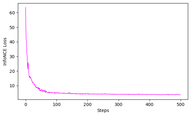
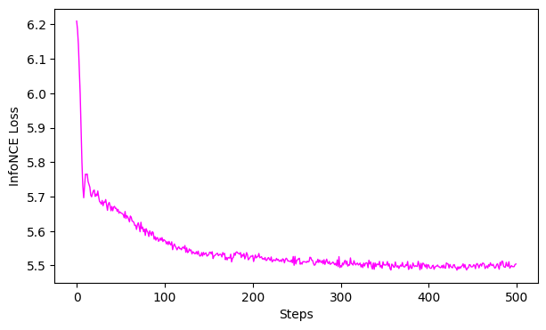
pos:  1.0293 neg:  2.6415 total:  3.6708 temperature:  1.1200: 100%|██████████| 500/500 [00:09<00:00, 50.92it/s]
pos: -0.8511 neg:  6.3554 total:  5.5043 temperature:  1.1200: 100%|██████████| 500/500 [00:08<00:00, 59.02it/s]

Let’s check the loss curve, examine the goodness of fit, then visualize the embedding

# 4. Evaluation
# GoFs
gof_full2D = cebra.sklearn.metrics.goodness_of_fit_score(cebra_time_full_model2D, dlc_data)
gof_full4D = cebra.sklearn.metrics.goodness_of_fit_score(cebra_time_full_model4D, dlc_data)
print(" GoF in bits - full 2D:", gof_full2D)
print(" GoF in bits - full 4D:", gof_full4D)
# plot the loss curves
ax = cebra.plot_loss(cebra_time_full_model2D)
ax = cebra.plot_loss(cebra_time_full_model4D)

100%|██████████| 500/500 [00:01<00:00, 263.90it/s]
100%|██████████| 500/500 [00:02<00:00, 229.79it/s]

 GoF in bits - full 2D: 3.5434484345827015
 GoF in bits - full 4D: 1.0726874258913286

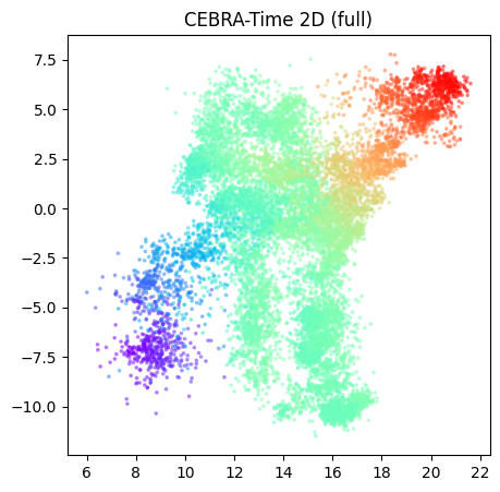
# 5. Visulization, 2D model:
fig = cebra.plot_embedding(cebra_time_full2D, embedding_labels=dlc_data[:,0],title = "CEBRA-Time 2D (full)", markersize=3, cmap = "rainbow")

# 5. Visulization, 3D+ model:

# plot embedding for outdim =>3:
fig = cebra.integrations.plotly.plot_embedding_interactive(cebra_time_full4D,
                                                           embedding_labels=dlc_data[:,0],
                                                           title = "CEBRA-Time (full)",
                                                           markersize=3,
                                                           cmap = "rainbow")
fig.show(renderer="notebook")

<Figure size 500x500 with 0 Axes>

Save the models 🦓

tmp_file2D = Path(tempfile.gettempdir(), 'cebra2D.pt')
tmp_file4D = Path(tempfile.gettempdir(), 'cebra4D.pt')
cebra_model2D.save(tmp_file2D)
cebra_model2D.save(tmp_file4D)
#reload one to check ✅
cebra_model = cebra.CEBRA.load(tmp_file2D)

🚧 To see the full range of options, including how to pick best parameters, please see the “Best practices” notebook!

Enjoy!