You can download and run the notebook locally or run it with Google Colaboratory:

---

Encoding of space: Co-homology and circular coordinates

In this notebook, we show how to:

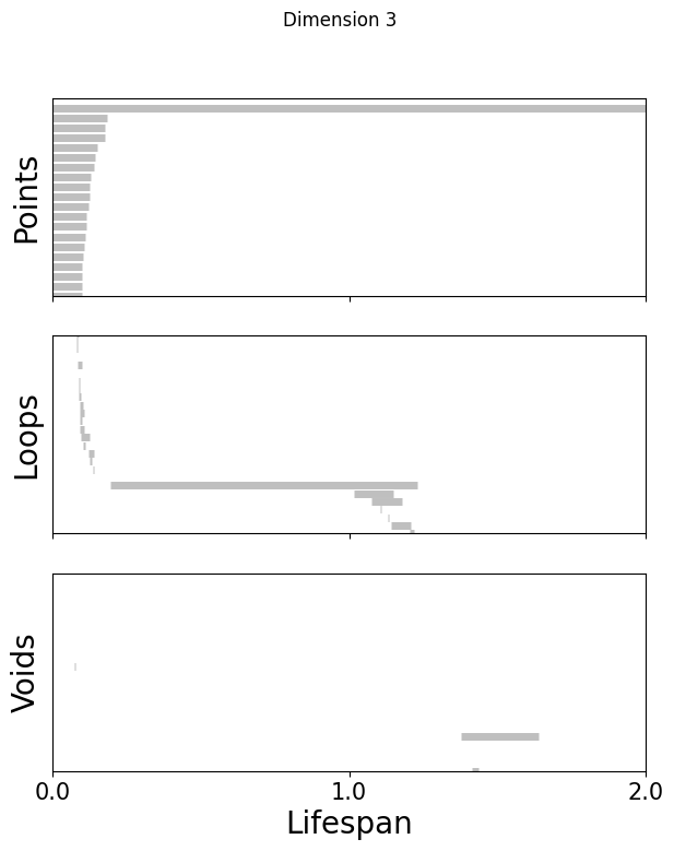
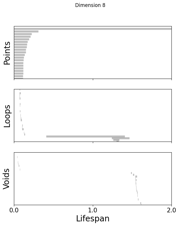
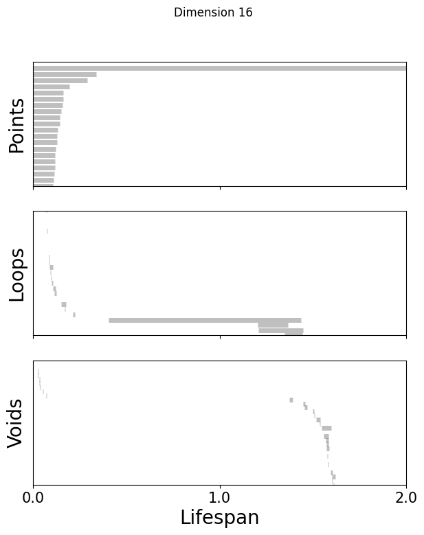
• perform persistent cohomology analysis to discover topological structure in the data.

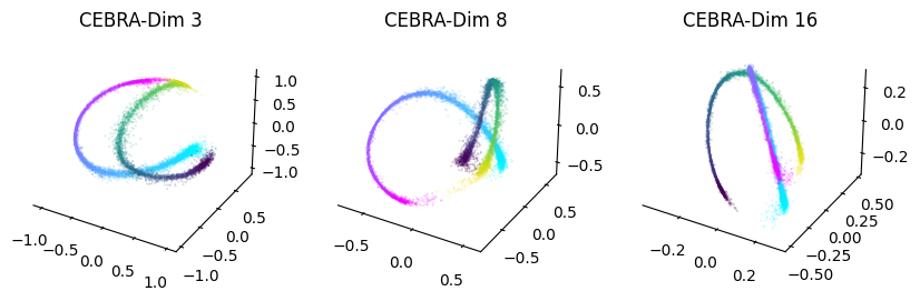
• visualize CEBRA embeddings into circular coordinates.

• explore the embeddings co-cycles.

For that we will compare CEBRA embeddings of varying output dimensions (3, 8, 16).

It is based in part from what was presented in Figure 2.e.-g. of Schneider, Lee, Mathis.

Install note

• Be sure you have cebra, and the demo dependencies, installed to use this notebook

!pip install --pre 'cebra[datasets,demos]'

import sys
import numpy as np
import matplotlib.pyplot as plt
import seaborn as sns
import pandas as pd
from matplotlib.collections import LineCollection

import cebra.datasets
import cebra
from cebra import CEBRA

Load the data:

• The data will be automatically downloaded into a /data folder.

hippocampus_pos = cebra.datasets.init('rat-hippocampus-single-achilles')

100%|██████████| 10.0M/10.0M [00:01<00:00, 8.99MB/s]

Download complete. Dataset saved in 'data/rat_hippocampus/achilles.jl'

——————- BEGINNING OF TRAINING SECTION ——————-

Train CEBRA-Behavior with different dimensions: 3, 8, 16

max_iterations = 10000 #default is 5000.

cebra_posdir3_model = CEBRA(model_architecture='offset10-model',
                        batch_size=512,
                        learning_rate=3e-4,
                        temperature=1,
                        output_dimension=3,
                        max_iterations=max_iterations,
                        distance='cosine',
                        conditional='time_delta',
                        device='cuda_if_available',
                        verbose=True,
                        time_offsets=10)

cebra_posdir8_model= CEBRA(model_architecture='offset10-model',
                        batch_size=512,
                        learning_rate=3e-4,
                        temperature=1,
                        output_dimension=8,
                        max_iterations=max_iterations,
                        distance='cosine',
                        conditional='time_delta',
                        device='cuda_if_available',
                        verbose=True,
                        time_offsets=10)

cebra_posdir16_model = CEBRA(model_architecture='offset10-model',
                        batch_size=512,
                        learning_rate=3e-4,
                        temperature=1,
                        output_dimension=16,
                        max_iterations=max_iterations,
                        distance='cosine',
                        conditional='time_delta',
                        device='cuda_if_available',
                        verbose=True,
                        time_offsets=10)

cebra_posdir3_model.fit(hippocampus_pos.neural, hippocampus_pos.continuous_index.numpy())
cebra_posdir3_model.save("cebra_posdir3_model.pt")

cebra_posdir8_model.fit(hippocampus_pos.neural, hippocampus_pos.continuous_index.numpy())
cebra_posdir8_model.save("cebra_posdir8_model.pt")

cebra_posdir16_model.fit(hippocampus_pos.neural, hippocampus_pos.continuous_index.numpy())
cebra_posdir16_model.save("cebra_posdir16_model.pt")

pos:  0.1023 neg:  5.4131 total:  5.5155 temperature:  1.0000: 100%|██████████| 10000/10000 [02:32<00:00, 65.75it/s]
pos:  0.1074 neg:  5.3878 total:  5.4952 temperature:  1.0000: 100%|██████████| 10000/10000 [02:33<00:00, 65.12it/s]
pos:  0.1003 neg:  5.3875 total:  5.4878 temperature:  1.0000: 100%|██████████| 10000/10000 [02:42<00:00, 61.61it/s]

——————- END OF TRAINING SECTION ——————-

Load the models and compute the embeddings

cebra_posdir3_model = cebra.CEBRA.load("cebra_posdir3_model.pt")
cebra_posdir3 = cebra_posdir3_model.transform(hippocampus_pos.neural)

cebra_posdir8_model = cebra.CEBRA.load("cebra_posdir8_model.pt")
cebra_posdir8 = cebra_posdir8_model.transform(hippocampus_pos.neural)

cebra_posdir16_model = cebra.CEBRA.load("cebra_posdir16_model.pt")
cebra_posdir16 = cebra_posdir16_model.transform(hippocampus_pos.neural)

Plot the results

right = hippocampus_pos.continuous_index[:,1] == 1
left = hippocampus_pos.continuous_index[:,2] == 1

fig = plt.figure(figsize = (10,3), dpi = 100)

ax1 = plt.subplot(131,projection='3d')
ax2 = plt.subplot(132, projection = '3d')
ax3 = plt.subplot(133, projection = '3d')

for dir, cmap in zip([right, left], ["cool", "viridis"]):
    ax1 = cebra.plot_embedding(ax=ax1, embedding=cebra_posdir3[dir,:], embedding_labels=hippocampus_pos.continuous_index[dir,0], cmap=cmap)
    ax2 = cebra.plot_embedding(ax=ax2, embedding=cebra_posdir8[dir,:], embedding_labels=hippocampus_pos.continuous_index[dir,0], cmap=cmap)
    ax3 = cebra.plot_embedding(ax=ax3, embedding=cebra_posdir16[dir,:], embedding_labels=hippocampus_pos.continuous_index[dir,0], cmap=cmap)

ax1.set_title('CEBRA-Dim 3')
ax2.set_title('CEBRA-Dim 8')
ax3.set_title('CEBRA-Dim 16')
plt.show()

Persistent cohomology analysis: topological data analysis

Get random 1000 points of the embeddings and do persistent cohomology analysis up to H1

• This requires the ripser package.

• If you previously installed DREiMac (such as running this notebook before, there are some dependency clashes with ripser, so you need to uninstall it first, and reinstall risper:

!pip uninstall -y dreimac
!pip uninstall -y cebra
!pip uninstall -y ripser

!pip install ripser

#Depending on your system, this can cause errors.
#Thus if issues please follow these instructions directly: https://pypi.org/project/ripser/
import ripser

If you get the error ValueError: numpy.ndarray size changed, may indicate binary incompatibility. Expected 96 from C header, got 80 from PyObject, please delete the folders from DREiMac and run the cell above again.

maxdim=1 # set to 2 to compute up to H2. The computing time is considerably longer.
         # For quick demo up to H1, set it to 1.
np.random.seed(111)
random_idx=np.random.permutation(np.arange(len(cebra_posdir3)))[:1000]
topology_dimension = {}
for embedding in [cebra_posdir3, cebra_posdir8, cebra_posdir16]:
    ripser_output=ripser.ripser(embedding[random_idx], maxdim=maxdim, coeff=47)
    dimension = embedding.shape[1]
    topology_dimension[dimension] = ripser_output

If you want to visualize the pre-computed persistent co-homology result:

Preloading saves quite a bit of time; to adapt to your own datasets please set topology_dimension and random_idx.

preload=pd.read_hdf(os.path.join(CURRENT_DIR,'rat_demo_example_output.h5'))
topology_dimension = preload['topology']
topology_random_dimension = preload['topology_random']
random_idx = preload['embedding']['random_idx']
maxdim=2

def plot_barcode(topology_result, maxdim):
    fig, axs = plt.subplots(maxdim+1, 1, sharex=True, figsize=(7, 8))
    axs[0].set_xlim(0,2)
    cocycle = ["Points", "Loops", "Voids"]
    for k in range(maxdim+1):
        bars = topology_result['dgms'][k]
        bars[bars == np.inf] = 10
        lc = (
            np.vstack(
                [
                    bars[:, 0],
                    np.arange(len(bars), dtype=int) * 6,
                    bars[:, 1],
                    np.arange(len(bars), dtype=int) * 6,
                ]
            )
            .swapaxes(1, 0)
            .reshape(-1, 2, 2)
        )
        line_segments = LineCollection(lc, linewidth=5, color="gray", alpha=0.5)
        axs[k].set_ylabel(cocycle[k], fontsize=20)
        if k == 0:
            axs[k].set_ylim(len(bars) * 6 - 120, len(bars) * 6)
        elif k == 1:
            axs[k].set_ylim(0, len(bars) * 1 - 30)
        elif k == 2:
            axs[k].set_ylim(0, len(bars) * 6 + 10)
        axs[k].add_collection(line_segments)
        axs[k].set_yticks([])
        if k == 2:
            axs[k].set_xticks(np.linspace(0, 2, 3), np
                              .linspace(0, 2, 3), fontsize=15)
            axs[k].set_xlabel("Lifespan", fontsize=20)

    return fig

%matplotlib inline
for k in [3,8,16]:
    fig=plot_barcode(topology_dimension[k], maxdim)
    fig.suptitle(f'Dimension {k}')

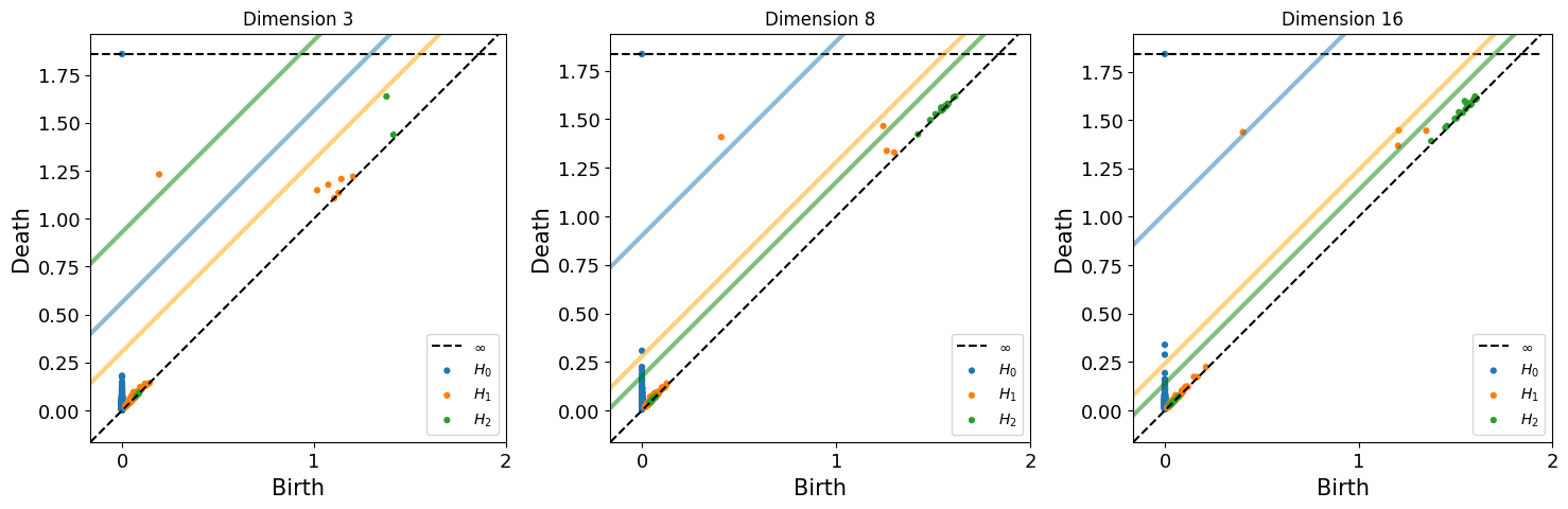
Compute the Betti numbers of the embeddings

The \(k^{th}\) Betti number refers to the number of k-dimensional holes on a topological surface. A “k-dimensional hole” is a k-dimensional cycle that is not a boundary of a (k+1)-dimensional object.

Informally, the Betti number refer to the number of times that an object can be “cut” before splitting into separate pieces.

from persim import plot_diagrams

def read_lifespan(ripser_output, dim):
    dim_diff = ripser_output['dgms'][dim][:, 1] - ripser_output['dgms'][dim][:, 0]
    if dim == 0:
        return dim_diff[~np.isinf(dim_diff)]
    else:
        return dim_diff

def get_max_lifespan(ripser_output_list, maxdim):
    lifespan_dic = {i: [] for i in range(maxdim+1)}
    for f in ripser_output_list:
        for dim in range(maxdim+1):
            lifespan = read_lifespan(f, dim)
            lifespan_dic[dim].extend(lifespan)
    return [max(lifespan_dic[i]) for i in range(maxdim+1)], lifespan_dic

def get_betti_number(ripser_output, shuffled_max_lifespan):
    bettis=[]
    for dim in range(len(ripser_output['dgms'])):
        lifespans=ripser_output['dgms'][dim][:, 1] - ripser_output['dgms'][dim][:, 0]
        betti_d = sum(lifespans > shuffled_max_lifespan[dim] * 1.1)
        bettis.append(betti_d)
    return bettis

def plot_lifespan(topology_dgms, shuffled_max_lifespan, ax, label_vis, maxdim):
    plot_diagrams(
        topology_dgms,
        ax=ax,
        legend=True,
    )

    ax.plot(
        [
            -0.5,
            2,
        ],
        [-0.5 + shuffled_max_lifespan[0], 2 + shuffled_max_lifespan[0]],
        color="C0",
        linewidth=3,
        alpha=0.5,

    )
    ax.plot(
        [
            -0.5,
            2,
        ],
        [-0.5 + shuffled_max_lifespan[1], 2 + shuffled_max_lifespan[1]],
        color="orange",
        linewidth=3,
        alpha=0.5,

    )
    if maxdim == 2:
        ax.plot(
            [-0.50, 2],
            [-0.5 + shuffled_max_lifespan[2], 2 + shuffled_max_lifespan[2]],
            color="green",
            linewidth=3,
            alpha=0.5,
        )
    ax.set_xlabel("Birth", fontsize=15)
    ax.set_xticks([0, 1, 2])
    ax.set_xticklabels([0, 1, 2])
    ax.tick_params(labelsize=13)
    if label_vis:
        ax.set_ylabel("Death", fontsize=15)
    else:
        ax.set_ylabel("")

fig = plt.figure(figsize=(18,5))
for n, dim in enumerate([3,8,16]):
    shuffled_max_lifespan, lifespan_dic = get_max_lifespan(topology_random_dimension[dim], maxdim)
    ax = fig.add_subplot(1,3,n+1)
    ax.set_title(f'Dimension {dim}')
    plot_lifespan(topology_dimension[dim]['dgms'], shuffled_max_lifespan, ax, True, maxdim)
    print(f"Betti No. for dimension {dim}: {get_betti_number(topology_dimension[dim], shuffled_max_lifespan)}")

Betti No. for dimension 3: [1, 1, 0]
Betti No. for dimension 8: [1, 1, 0]
Betti No. for dimension 16: [1, 1, 0]

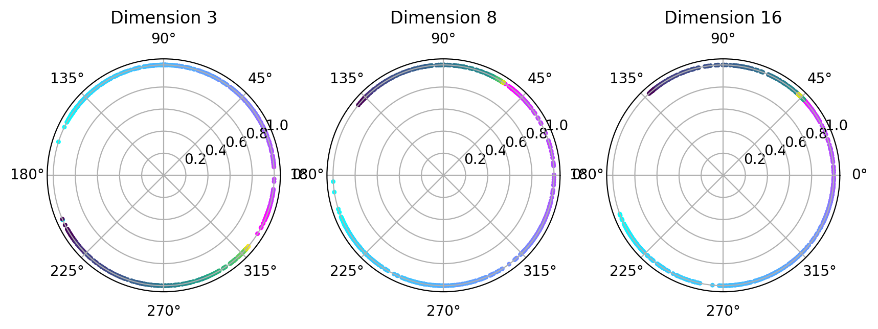
Visualize topology-preserving circular coordinates from the first co-cycle.

This requires the DREiMac codebase. Here, we show you how to install their package:

!pip install git+https://github.com/ctralie/DREiMac.git@cdd6d02ba53c3597a931db9da478fd198d6ed00f

from dreimac import CircularCoords

%matplotlib inline

prime = 47
dimension = [3,8,16]
fig, axs = plt.subplots(1, 3, figsize=(10,3), dpi=200, subplot_kw={'projection': 'polar'})
label = hippocampus_pos.continuous_index[random_idx]
r_ind = label[:,1]==1
l_ind = label[:,2]==1
for i, embedding in enumerate([cebra_posdir3, cebra_posdir8, cebra_posdir16]):
    rat_emb=embedding[random_idx]
    cc = CircularCoords(rat_emb, 1000, prime = prime, )
    radial_angle=cc.get_coordinates(cocycle_idx=[0])
    r = np.ones(1000)
    right=axs[i].scatter(radial_angle[r_ind], r[r_ind], s=5, c = label[r_ind,0], cmap = 'cool')
    left=axs[i].scatter(radial_angle[l_ind], r[l_ind], s=5, c = label[l_ind,0], cmap = 'viridis')
    axs[i].set_title(f'Dimension {dimension[i]}')
plt.show()

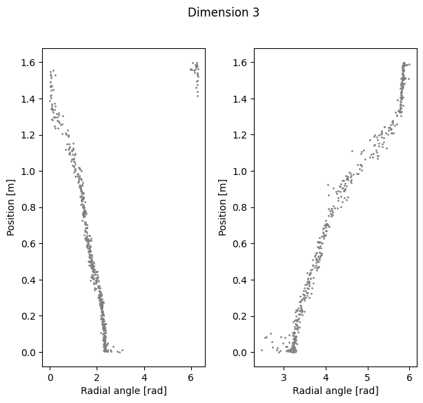
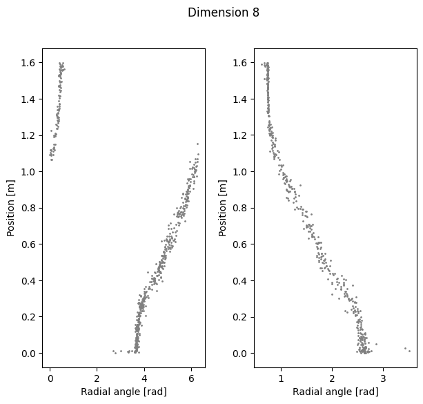
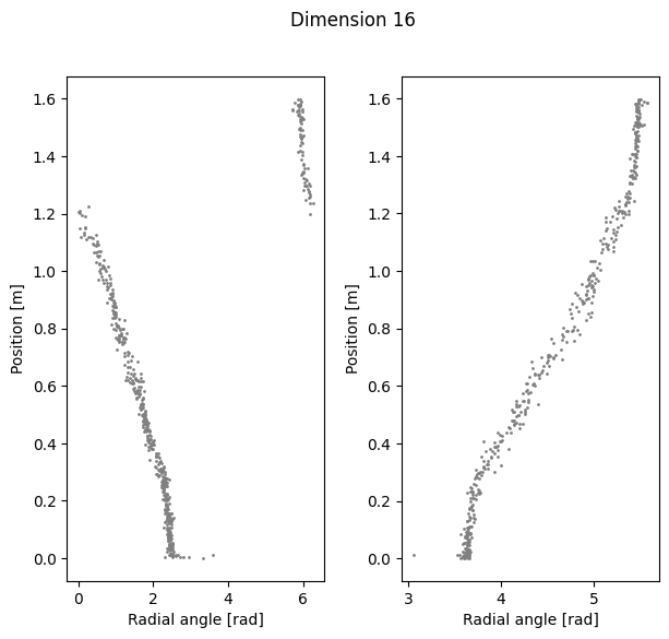
Visualize polar coordinate (radial angle)

If you want to preload our data, run the following, otherwise skip this cell:

cebra_pos3 = preload['embedding'][3]
cebra_pos8 = preload['embedding'][8]
cebra_pos16 = preload['embedding'][16]

radial_angles = {}
for i, embedding in enumerate([cebra_pos3, cebra_pos8, cebra_pos16]):
    rat_emb=embedding[random_idx]
    cc = CircularCoords(rat_emb, 1000, prime = prime, )
    out=cc.get_coordinates()
    radial_angles[dimension[i]] = out

%matplotlib inline
for k in radial_angles.keys():
    fig=plt.figure(figsize=(7,6))
    plt.subplots_adjust(wspace=0.3)
    fig.suptitle(f'Dimension {k}')
    ax1=plt.subplot(121)
    ax1.scatter(radial_angles[k][r_ind], label[r_ind,0], s=1, c = 'gray')
    ax1.set_xlabel('Radial angle [rad]')
    ax1.set_ylabel('Position [m]')
    ax2=plt.subplot(122)
    ax2.scatter(radial_angles[k][l_ind], label[l_ind,0], s=1, c= 'gray')
    ax2.set_xlabel('Radial angle [rad]')
    ax2.set_ylabel('Position [m]')
plt.show()

Compute linear correlation between computed polar coordinates and position

import sklearn.linear_model
def lin_regression(radial_angles, labels):
    def _to_cartesian(radial_angles):
        x = np.cos(radial_angles)
        y = np.sin(radial_angles)
        return np.vstack([x,y]).T
    cartesian = _to_cartesian(radial_angles)
    lin = sklearn.linear_model.LinearRegression()
    lin.fit(cartesian, labels)

    return lin.score(cartesian, labels)

for k in radial_angles.keys():
    print(f'Dimension {k} Cycle angle into position')
    print(f'Right R2: {lin_regression(radial_angles[k][r_ind], label[r_ind,0])}')
    print(f'Left R2: {lin_regression(radial_angles[k][l_ind], label[l_ind,0])}')
    print(f'Total R2: {lin_regression(radial_angles[k], label[:,0])}')

Dimension 3 Cycle angle into position
Right R2: 0.9786339781977732
Left R2: 0.9636014502747399
Total R2: 0.9563695397160188
Dimension 8 Cycle angle into position
Right R2: 0.9288158799657967
Left R2: 0.9607563744350794
Total R2: 0.892921888751599
Dimension 16 Cycle angle into position
Right R2: 0.9614739746985121
Left R2: 0.9702177580250442
Total R2: 0.949558194067378

Interactive plot to explore co-cycles and circular coordinates.

• Top left panel is a lifespan diagram of persistent co-homology analysis.

• Bottom left panel is a visualization of the first 2 dimensions of the used 1000 embedding points.

• Bottom right panel is a circular coordinate obtained from the co-cycles.

• For more information: ctralie/DREiMac

Note to Google Colaboratory users: replace the first line of the next cell (%matplotlib notebook) with %matplotlib inline.

## change the embedding to use. Here, we look at 3D embedding for posdir3 (position+dir, dim 3):
X=cebra_posdir3[random_idx]

%matplotlib notebook
rl_stack=np.vstack([X[r_ind], X[l_ind]])
label_stack = np.vstack([label[r_ind], label[l_ind]])

c1 = plt.get_cmap('cool')
C1 = c1(label[r_ind,0])
c2 = plt.get_cmap('viridis')
C2 = c2(label[l_ind,0])

C = np.vstack([C1,C2])

def plot_circles(ax):
    ax.scatter(rl_stack[:, 0], rl_stack[:, 1], c=C)


cc = CircularCoords(rl_stack, 1000, prime = prime)
cc.plot_torii(C, coords_info=2, plots_in_one=3, lowerleft_plot=plot_circles)

/home/celia/miniconda3/envs/cebra/lib/python3.10/site-packages/dreimac/emcoords.py:66: UserWarning: Could not accurately determine screen size
  warnings.warn("Could not accurately determine screen size")