Using CEBRA

This page covers a standard CEBRA usage. We recommend checking out the Demo Notebooks for CEBRA usage examples as well. Here we present a quick overview on how to use CEBRA on various datasets. Note that we provide two ways to interact with the code:

• For regular usage, we recommend leveraging the high-level interface, adhering to scikit-learn formatting.

• Upon specific needs, advanced users might consider diving into the low-level interface that adheres to PyTorch formatting.

Firstly, why use CEBRA?

CEBRA is primarily designed for producing robust, consistent extractions of latent factors from time-series data. It supports three modes, and is a self-supervised representation learning algorithm that uses our modified contrastive learning approach designed for multi-modal time-series data. In short, it is a type of non-linear dimensionality reduction, like tSNE and UMAP. We show in our original paper that it outperforms tSNE and UMAP at producing closer-to-ground-truth latents and is more consistent.

That being said, CEBRA can be used on non-time-series data and it does not strictly require multi-modal data. In general, we recommend considering using CEBRA for measuring changes in consistency across conditions (brain areas, cells, animals), for hypothesis-guided decoding, and for topological exploration of the resulting embedding spaces. It can also be used for visualization and considering dynamics within the embedding space. For examples of how CEBRA can be used to map space, decode natural movies, and make hypotheses for neural coding of sensorimotor systems, see Schneider, Lee, Mathis. Nature 2023.

The CEBRA workflow

CEBRA supports three modes: fully unsupervised (CEBRA-Time), supervised (via joint modeling of auxiliary variables; CEBRA-Behavior), and a hybrid variant (CEBRA-Hybrid). We recommend to start with running CEBRA-Time (unsupervised) and look both at the loss value (goodness-of-fit) and visualize the embedding. Then use labels via CEBRA-Behavior to test which labels give you this goodness-of-fit (tip: see our Figure 2: Hypothesis-driven and discovery-driven analysis with CEBRA hippocampus data example). Notably, if you use CEBRA-Behavior with labels that are not encoded in your data, the embedding will collapse (not-converged). This is a feature, not a bug. This allows you to rule out which obervable behaviors (labels) are truly in your data. To get a sense of this workflow, you can also look at Figure 2: Hypothesis-driven and discovery-driven analysis with CEBRA and Extended Data Figure 5: Hypothesis testing with CEBRA.. 👉 Here is a quick-start workflow, with many more details below:

1. Use CEBRA-Time for unsupervised data exploration.

2. Consider running a hyperparameter sweep on the inputs to the model, such as cebra.CEBRA.model_architecture, cebra.CEBRA.time_offsets, cebra.CEBRA.output_dimension, and set cebra.CEBRA.batch_size to be as high as your GPU allows. You want to see clear structure in the 3D plot (the first 3 latents are shown by default).

3. Use CEBRA-Behavior with many different labels and combinations, then look at the InfoNCE loss - the lower the loss value, the better the fit (see Extended Data Figure 5: Hypothesis testing with CEBRA.), and visualize the embeddings. The goal is to understand which labels are contributing to the structure you see in CEBRA-Time, and improve this structure. Again, you should consider a hyperparameter sweep (and avoid overfitting by performing the proper train/validation split (see Step 3 in our quick start guide below).

4. Interpretability: now you can use these latents in downstream tasks, such as measuring consistency, decoding, and determining the dimensionality of your data with topological data analysis.

All the steps to do this are described below. Enjoy using CEBRA! 🔥🦓

Step-by-step CEBRA

For a quick start into applying CEBRA to your own datasets, we provide a scikit-learn compatible API, similar to methods such as tSNE, UMAP, etc. We assume you have CEBRA installed in the environment you are working in, if not go to the Installation Guide. Next, launch your conda env (e.g., conda activate cebra).

Create a CEBRA workspace

Assuming you have your data recorded, you want to start using CEBRA on it. For instance you can create a new jupyter notebook.

For the sake of this usage guide, we create some example data:

# Create a .npz file
import numpy as np

X = np.random.normal(0,1,(100,3))
X_new = np.random.normal(0,1,(100,4))
np.savez("neural_data", neural = X, new_neural = X_new)

# Create a .h5 file, containing a pd.DataFrame
import pandas as pd

X_continuous = np.random.normal(0,1,(100,3))
X_discrete = np.random.randint(0,10,(100, ))
df = pd.DataFrame(np.array(X_continuous), columns=["continuous1", "continuous2", "continuous3"])
df["discrete"] = X_discrete
df.to_hdf("auxiliary_behavior_data.h5", key="auxiliary_variables")

You can start by importing the CEBRA package, as well as the CEBRA model as a classical scikit-learn estimator.

import cebra
from cebra import CEBRA

Data loading

Get the data ready

We acknowledge that your data can come in all formats. That is why we developed a loading helper function to help you get your data ready to be used by CEBRA.

The function cebra.load_data() supports various file formats to convert the data of interest to a numpy.array(). It handles three categories of data. Note that it will only read the data of interest and output the corresponding numpy.array(). It does not perform pre-processing so your data should be ready to be used for CEBRA.

• Your data is a 2D array. In that case, we handle Numpy, HDF5, PyTorch, csv, Excel, Joblib, Pickle and MAT-files. If your file only containsyour data then you can use the default cebra.load_data(). If your file contains more than one dataset, you will have to provide a key, which corresponds to the data of interest in the file.

• Your data is a pandas.DataFrame. In that case, we handle HDF5 files only. Similarly, you can use the default cebra.load_data() if your file only contains a single dataset and you want to get the whole pandas.DataFrame as your dataset. Else, if your file contains more than one dataset, you will have to provide the corresponding key. Moreover, if your pandas.DataFrame is a single index, you can precise the columns to fetch from the pandas.DataFrame for your data of interest.

In the following example, neural_data.npz contains multiple numpy.array() and auxiliary_behavior_data.h5, multiple pandas.DataFrame.

import cebra

# Load the .npz
neural_data = cebra.load_data(file="neural_data.npz", key="neural")

# ... and similarly load the .h5 file, providing the columns to keep
continuous_label = cebra.load_data(file="auxiliary_behavior_data.h5", key="auxiliary_variables", columns=["continuous1", "continuous2", "continuous3"])
discrete_label = cebra.load_data(file="auxiliary_behavior_data.h5", key="auxiliary_variables", columns=["discrete"]).flatten()

You can then use neural_data, continuous_label or discrete_label directly as the input or index data of your CEBRA model. Note that we flattened discrete_label in order to get a 1D numpy.array() as required for discrete index inputs.

Note

cebra.load_data() only handles one set of data at a time, either the data or the labels, for one session only. To use multiple sessions and/or multiple labels, the function can be called for each of dataset. For files containing multiple matrices, the corresponding key, referenciating the dataset in the file, must be provided.

See API docs: cebra.load_data()

cebra.load_data(file, key=None, columns=None)

Load a dataset from the given file.

The following file types are supported:

• Numpy files: npy, npz;

• HDF5 files: h5, hdf, hdf5, including h5 generated through DLC;

• PyTorch files: pt, p;

• csv files;

• Excel files: xls, xlsx, xlsm;

• Joblib files: jl;

• Pickle files: p, pkl;

• MAT-files: mat.

The assumptions on your data are as following:

• it contains at least one data structure (e.g. a numpy array, a torch.Tensor, etc.);

• it can be directly in the form of a collection (e.g. a dictionary);

• if the file contains a collection, the user can provide a key to refer to the data value they want to access;

• if no key is provided, the first data structure found upon iteration of the collection will be loaded;

• if a key is provided, it needs to correspond to an existing item of the collection;

• if a key is provided, the data value accessed needs to be a data structure;

• the function loads data for only one data structure, even if the file contains more. The function can be called again with the corresponding key to get the other ones.

Parameters:

• file (Union[str, Path]) – The path to the given file to load, in a supported format.

• key (Union[str, int, None]) – The key referencing the data of interest in the file, if the file has a dictionary-like structure.

• columns (Optional[list]) – The part of the data to keep in the output 2D-array. For now, it corresponds to the columns of a DataFrame to keep if the data selected is a DataFrame.

Return type:

ndarray[tuple[int, ...], dtype[TypeVar(_ScalarType_co, bound= generic, covariant=True)]]

Returns:

The loaded data.

Example

>>> import cebra
>>> import cebra.helper as cebra_helper
>>> import numpy as np
>>> # Create the files to load the data from
>>> # Create a .npz file
>>> X = np.random.normal(0,1,(100,3))
>>> y = np.random.normal(0,1,(100,4))
>>> np.savez("data", neural = X, trial = y)
>>> # Create a .h5 file
>>> url = "https://github.com/DeepLabCut/DeepLabCut/blob/main/examples/Reaching-Mackenzie-2018-08-30/labeled-data/reachingvideo1/CollectedData_Mackenzie.h5?raw=true"
>>> dlc_file = cebra_helper.download_file_from_url(url) # an .h5 example file
>>> # Load data
>>> X = cebra.load_data(file="data.npz", key="neural")
>>> y_trial_id = cebra.load_data(file="data.npz", key="trial")
>>> y_behavior = cebra.load_data(file=dlc_file, columns=["Hand", "Tongue"])

See API docs: cebra.load_deeplabcut()

cebra.load_deeplabcut(filepath, keypoints=None, pcutoff=0.6)

Load DLC data from h5 files.

Parameters:

• filepath (Union[Path, str]) – Path to the .h5 file containing DLC output data.

• keypoints (Optional[list]) – List of keypoints to keep in the output numpy.array.

• pcutoff (float) – Drop-out threshold. If the likelihood value on the estimated positions a sample is smaller than that threshold, then the sample is set to nan. Then, the nan values are interpolated.

Return type:

ndarray[tuple[int, ...], dtype[TypeVar(_ScalarType_co, bound= generic, covariant=True)]]

Returns:

A 2D array (n_samples x n_features) containing the data (x and y) generated by DLC for each keypoint of interest. Note that the likelihood is dropped.

Example

>>> import cebra
>>> url = ANNOTATED_DLC_URL = "https://github.com/DeepLabCut/DeepLabCut/blob/main/examples/Reaching-Mackenzie-2018-08-30/labeled-data/reachingvideo1/CollectedData_Mackenzie.h5?raw=true"
>>> file = cebra.helper.download_file_from_url(url) # an .h5 example file
>>> dlc_data = cebra.load_deeplabcut(file, keypoints=["Hand", "Joystick1"], pcutoff=0.6)

Choose the CEBRA mode and related auxiliary variables

CEBRA allows you to jointly use time-series data and (optionally) auxiliary variables to extract latent spaces. If you want to use time-only (namely, unsupervised) select:

• CEBRA-Time: Discovery-driven: time contrastive learning. Set conditional='time'. No assumption on the behaviors that are influencing neural activity. It can be used as a first step into the data analysis for instance, or as a comparison point to multiple hypothesis-driven analyses.

To use auxiliary (behavioral) variables you can choose both continuous and discrete variables. The label information (none, discrete, continuous) determine the algorithm to use for data sampling. Using labels allows you to project future behavior onto past time-series activity, and explicitly use label-prior to shape the embedding. The conditional distribution can be chosen upon model initialization with the cebra.CEBRA.conditional parameter.

• CEBRA-Behavior: Hypothesis-driven: behavioral contrastive learning. Set conditional='time_delta'. The user makes an hypothesis on the variables influencing neural activity (behavioral features such as position or head orientation, trial number, brain region, etc.). If the chosen auxiliary variables are in fact influencing the data to reduce, the resulting embedding should reflect that. Hence, it can easily be used to compare hypotheses. Auxiliary variables can be multiple, and both continuous and discrete. 👉 Examples on how to select them are presented in Forelimb dynamics, somatosensory (S1).

  • Discrete auxiliary variables. A 1D matrix, containing int. Example: trial ID, rewards, brain region ID.

    Note

    There can be only one discrete set of index per model.

  • Continuous auxiliary variables. A 2D matrix, containing float. Multiple continuous index can be chosen for the same model. Example: kinematics, actions.

• CEBRA-Hybrid: hybrid contrastive learning, using both time and behavioral variables. Set conditional='time_delta' and hybrid=True.

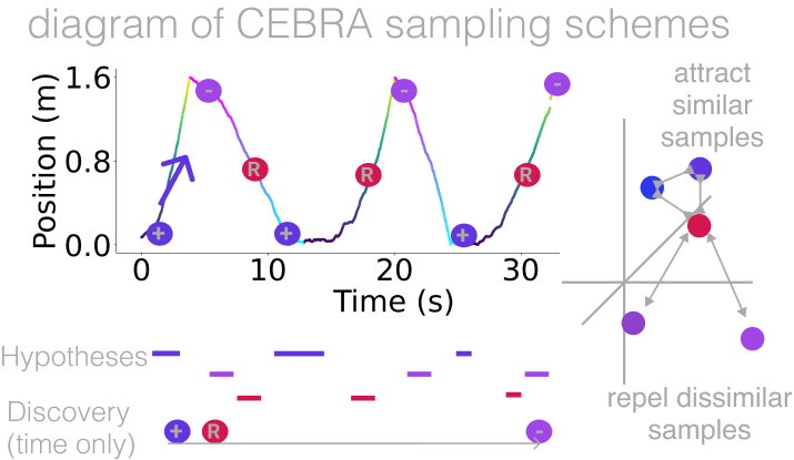
CEBRA sampling schemes: discovery-driven, hypothesis-driven, or in a hybrid mode. In the hypothesis-driven mode, the positive and negative samples are found based on the reference samples.

👉 Examples on how to use each of the conditional distribution and how to compare them when analyzing data are presented in Encoding of space, hippocampus (CA1).

Model definition

CEBRA training is modular, and model fitting can serve different downstream applications and research questions. Here, we describe how you can adjust the parameters depending on your data type and the hypotheses you might have.

Model architecture model_architecture

We provide a set of pre-defined models. You can access (and search) a list of available pre-defined models by running:

import cebra.models
print(cebra.models.get_options('offset*', limit = 4))

['offset10-model', 'offset10-model-mse', 'offset5-model', 'offset1-model-mse']

Then, you can choose the one that fits best with your needs and provide it to the CEBRA model as the model_architecture parameter.

As an indication the table below presents the model architecture we used to train CEBRA on the datasets presented in our paper (Schneider, Lee, Mathis. Nature 2023).

Dataset	Data type	Brain area	Model architecture
Artificial spiking	Synthetic		‘offset1-model-mse’
Rat hippocampus	Electrophysiology	CA1 hippocampus	‘offset10-model’
Macaque	Electrophysiology	Somatosensory cortex (S1)	‘offset10-model’
Allen Mouse	Calcium imaging (2P)	Visual cortex	‘offset10-model’
Allen Mouse	Neuropixels	Visual cortex	‘offset40-model-4x-subsample’

🚀 Optional: design your own model architectures

It is possible to construct a personalized model and use the @cebra.models.register decorator on it. For example:

from torch import nn
import cebra.models
import cebra.data
from cebra.models.model import _OffsetModel, ConvolutionalModelMixin

@cebra.models.register("my-model") # --> add that line to register the model!
class MyModel(_OffsetModel, ConvolutionalModelMixin):

    def __init__(self, num_neurons, num_units, num_output, normalize=True):
        super().__init__(
            nn.Conv1d(num_neurons, num_units, 2),
            nn.GELU(),
            nn.Conv1d(num_units, num_units, 40),
            nn.GELU(),
            nn.Conv1d(num_units, num_output, 5),
            num_input=num_neurons,
            num_output=num_output,
            normalize=normalize,
        )

    # ... and you can also redefine the forward method,
    # as you would for a typical pytorch model

    def get_offset(self):
        return cebra.data.Offset(22, 23)

# Access the model
print(cebra.models.get_options('my-model'))

Once your personalized model is defined, you can use by setting model_architecture='my-model'. 👉 See the Models and Criteria API for more details.

Criterion and distance criterion and distance

For standard usage we recommend the default values (i.e., InfoNCE and cosine respectively) which are specifically designed for our contrastive learning algorithms.

Conditional distribution conditional

👉 See the previous section on how to choose the auxiliary variables and a conditional distribution.

Note

If the auxiliary variables types do not match with conditional, the model training will fall back to time contrastive learning.

Temperature temperature

temperature has the largest effect on visualization of the embedding (see Extended Data Figure 2: Hyperparameter changes on visualization and consistency.). Hence, it is important that it is fitted to your specific data. Lower temperatures (e.g. around 0.1) will result in a more dispersed embedding, higher temperatures (larger than 1) will concentrate the embedding.

🚀 For advance usage, you might need to find the optimal temperature. For that we recommend to perform a grid-search.

👉 More examples on how to handle temperature can be found in Technical: Learning the temperature parameter.

Time offsets \(\Delta\) time_offsets

This corresponds to the distance (in time) between positive pairs and informs the algorithm about the time-scale of interest.

The interpretation of this parameter depends on the chosen conditional distribution. A higher time offset typically will increase the difficulty of the learning task, and (within a range) improve the quality of the representation. For time-contrastive learning, we generally recommend that the time offset should be larger than the specified receptive field of the model.

Number of iterations max_iterations

We recommend to use at least 10,000 iterations to train the model. For prototyping, it can be useful to start with a smaller number (a few 1,000 iterations). However, when you notice that the loss function does not converge or the embedding looks uniformly distributed (cloud-like), we recommend increasing the number of iterations.

Note

You should always assess the convergence of your model at the end of training by observing the training loss (see Visualize the training loss).

Number of adaptation iterations max_adapt_iterations

One feature of CEBRA is you can apply (adapt) your model to new data. If you are planning to adapt your trained model to a new set of data, we recommend to use around 500 steps to re-tuned the first layer of the model.

In the paper, we show that fine-tuning the input embedding (first layer) on the novel data while using a pretrained model can be done with 500 steps in 3.5s only, and has better performance overall.

Batch size batch_size

CEBRA should be trained on the biggest batch size possible. Ideally, and depending on the size of your dataset, you should set batch_size to None (default value) which will train the model drawing samples from the full dataset at each iteration. As an indication, all the models used in the paper were trained with batch_size=512. You should avoid having to set your batch size to a smaller value.

Warning

Using the full dataset (batch_size=None) is only implemented for single-session training with continuous auxiliary variables.

Here is an example of a CEBRA model initialization:

cebra_model = CEBRA(
    model_architecture = "offset10-model",
    batch_size = 1024,
    learning_rate = 0.001,
    max_iterations = 10,
    time_offsets = 10,
    output_dimension = 8,
    device = "cuda_if_available",
    verbose = False
)

print(cebra_model)

CEBRA(batch_size=1024, learning_rate=0.001, max_iterations=10,
      model_architecture='offset10-model', time_offsets=10)

See API docs

class cebra.CEBRA(model_architecture='offset1-model', device='cuda_if_available', criterion='infonce', distance='cosine', conditional=None, temperature=1.0, temperature_mode='constant', min_temperature=0.1, time_offsets=1, delta=None, max_iterations=10000, max_adapt_iterations=500, batch_size=None, learning_rate=0.0003, optimizer='adam', output_dimension=8, verbose=False, num_hidden_units=32, pad_before_transform=True, hybrid=False, optimizer_kwargs=(('betas', (0.9, 0.999)), ('eps', 1e-08), ('weight_decay', 0), ('amsgrad', False)))

Bases: TransformerMixin, BaseEstimator

CEBRA model defined as part of a scikit-learn-like API.

model_architecture

The architecture of the neural network model trained with contrastive learning to encode the data. We provide a list of pre-defined models which can be displayed by running cebra.models.get_options(). The user can also register their own custom models (see in Docs).

Default: offset1-model

Type:

str

device

The device used for computing. Choose from cpu, cuda, cuda_if_available' or a particular GPU via cuda:0.

Default: cuda_if_available

Type:

str

criterion

The training objective. Currently only the default InfoNCE is supported. The InfoNCE loss is specifically designed for contrastive learning.

Default: InfoNCE

Type:

str

distance

The distance function used in the training objective to define the positive and negative samples with respect to the reference samples. Currently supports cosine and euclidean distances, cosine being specifically adapted for contrastive learning.

Default: cosine

Type:

str

conditional

The conditional distribution to use to sample the positive samples. Reference and negative samples are drawn from a uniform prior. For positive samples, it currently supports 3 types of distributions: time_delta, time and delta. Positive sample are distributed around the reference samples using either time information (time) with a fixed time_offset from the reference samples’ time steps, or the auxililary variables, considering the empirical distribution of how behavior vary across time_offset timesteps (time_delta). Alternatively (delta), the distribution is set as a Gaussian distribution, parametrized by a fixed delta around the reference sample.

Default: None

Type:

str

temperature

Factor by which to scale the similarity of the positive and negative pairs in the InfoNCE loss. Higher values yield “sharper”, more concentrated embeddings.

Default: 1.0

Type:

float

temperature_mode

The constant mode uses a temperature set by the user, constant during training. The auto mode trains the temperature alongside the model. If set to auto. In that case, make sure to also set min_temperature to a value in the expected range (for that a simple grid-search over temperature can be run). Note that the auto mode is an experimental feature for now.

Default: constant

Type:

str

min_temperature

The minimum temperature to maintain in case the temperature is optimized with the model (when setting temperature_mode to auto). This parameter will be ignored if temperature_mode is set to constant. Select None if no constraint should be applied.

Default: 0.1

Type:

float

time_offsets

The offsets for building the empirical distribution within the chosen sampler. It can be a single value, or a tuple of values to sample from uniformly. Will only have an effect if conditional is set to time or time_delta.

Type:

int

max_iterations

The number of iterations to train for. To pick the optimal number of iterations, start with a lower number (like 1,000) for faster training, and observe the value of the loss function (see plot_loss() to display the model loss over training). Make sure to pick a number of iterations high enough for the loss to converge.

Default: 10000.

Type:

int

max_adapt_iterations

The number of samples for retraining the first layer when adapting the model to a new dataset. This parameter is only relevant when adapt=True in cebra.CEBRA.fit().

Default: 500.

Type:

int

batch_size

The batch size to use for training. If RAM or GPU memory allows, this parameter can be set to None to select batch gradient descent on the whole dataset. If you use mini-batch training, you should aim for a value greater than 512. Higher values typically get better results and smoother loss curves.

Default: None.

Type:

int

learning_rate

The learning rate for optimization. Higher learning rates can yield faster convergence, but also lead to instability. Tune this parameter along with :py:attr:~.temperature`. For stable training with lower temperatures, it can make sense to lower the learning rate, and train a bit longer.

Default: 0.0003.

Type:

float

optimizer

The optimizer to use. Refer to torch.optim for all possible optimizers. Right now, only adam is supported.

Default: adam.

Type:

str

output_dimension

The output dimensionality of the embedding. For visualization purposes, this can be set to 3 for an embedding based on the cosine distance and 2-3 for an embedding based on the Eulidean distance (see distance). Alternatively, fit an embedding with a higher output dimensionality and then perform a linear ICA on top to visualize individual components.

Default: 8.

Type:

int

verbose

If True, show a progress bar during training.

Default: False.

Type:

bool

num_hidden_units

The number of dimensions to use within the neural network model. Higher numbers slow down training, but make the model more expressive and can result in a better embedding. Especially if you find that the embeddings are not consistent across runs, increase num_hidden_units and output_dimension to increase the model size and output dimensionality.

Default: 32.

Type:

int

pad_before_transform

If False, the output sequence will be smaller than the input sequence due to the receptive field of the model. For example, if the input sequence is 100 steps long, and a model with receptive field 10 is used, the output sequence will only be 100-10+1 steps long. For typical use cases, this parameters can be left at the default.

Default: True.

Type:

bool

hybrid

If True, the model will be trained using both the time-contrastive and the selected behavior-constrastive loss functions.

Default: False.

Type:

bool

optimizer_kwargs

Additional optimization parameters. These have the form ((key, value), (key, value)) and are passed to the PyTorch optimizer specified through the optimizer argument. Refer to the optimizer documentation in torch.optim for further information on how to format the arguments.

Default: (('betas', (0.9, 0.999)), ('eps', 1e-08), ('weight_decay', 0), ('amsgrad', False))

Type:

dict

Example

>>> import cebra
>>> cebra_model = cebra.CEBRA(model_architecture='offset10-model',
...                           batch_size=512,
...                           learning_rate=3e-4,
...                           temperature=1,
...                           output_dimension=3,
...                           max_iterations=10,
...                           distance='cosine',
...                           conditional='time_delta',
...                           device='cuda_if_available',
...                           verbose=True,
...                           time_offsets = 10)

Model training

Single-session versus multi-session training

We provide both single-sesison and multi-session training. The latest makes the resulting embeddings invariant to the auxiliary variables across all sessions.

Note

For flexibility reasons, the multi-session training fits one model for each session and thus sessions don’t necessarily have the same number of features (e.g., number of neurons).

Check out the following list to verify if the multi-session implementation is the right tool for your needs.

I have multiple sessions/animals that I want to consider as a pseudo-subject and use them jointly for training CEBRA. That is the case because of limited access to simultaneously recorded neurons or looking for animal-invariant features in the neural data.

I want to get more consistent embeddings from one session/animal to the other.

I want to be able to use CEBRA for a new session that is fully unseen during training.

Warning

Using multi-session training limits the influence of individual variations per session on the embedding. Make sure that this session/animal-specific information won’t be needed in your downstream analysis.

👉 Have a look at Technical: Training models across animals for more in-depth usage examples of the multi-session training.

Training

Single-session training

CEBRA is trained using cebra.CEBRA.fit(), similarly to the examples below for single-session training, using cebra_model as defined above. You can pass the input data as well as the behavioral labels you selected.

timesteps = 5000
neurons = 50
out_dim = 8

neural_data = np.random.normal(0,1,(timesteps, neurons))
continuous_label = np.random.normal(0,1,(timesteps, 3))
discrete_label = np.random.randint(0,10,(timesteps,))

single_cebra_model = cebra.CEBRA(batch_size=512,
                                 output_dimension=out_dim,
                                 max_iterations=10,
                                 max_adapt_iterations=10)

Note that the discrete_label array needs to be one dimensional, and needs to be of type int.

We can now fit the model in different modes.

• For CEBRA-Time (time-contrastive training) with the chosen time_offsets, run:

single_cebra_model.fit(neural_data)

• For CEBRA-Behavior (supervised constrastive learning) using discrete labels, run:

single_cebra_model.fit(neural_data, discrete_label)

• For CEBRA-Behavior (supervised constrastive learning) using continuous labels, run:

single_cebra_model.fit(neural_data, continuous_label)

• For CEBRA-Behavior (supervised constrastive learning) using a mix of discrete and continuous labels, run

single_cebra_model.fit(neural_data, continuous_label, discrete_label)

Multi-session training

For multi-session training, lists of data are provided instead of a single dataset and eventual corresponding auxiliary variables.

Warning

For now, multi-session training can only handle a unique set of continuous labels or a unique discrete label. All other combinations will raise an error. For the continuous case we provide the following example:

timesteps1 = 5000
timesteps2 = 3000
neurons1 = 50
neurons2 = 30
out_dim = 8

neural_session1 = np.random.normal(0,1,(timesteps1, neurons1))
neural_session2 = np.random.normal(0,1,(timesteps2, neurons2))
continuous_label1 = np.random.uniform(0,1,(timesteps1, 3))
continuous_label2 = np.random.uniform(0,1,(timesteps2, 3))

multi_cebra_model = cebra.CEBRA(batch_size=512,
                                output_dimension=out_dim,
                                max_iterations=10,
                                max_adapt_iterations=10)

Once you defined your CEBRA model, you can run:

multi_cebra_model.fit([neural_session1, neural_session2], [continuous_label1, continuous_label2])

Similarly, for the discrete case a discrete label can be provided and the CEBRA model will use the discrete multisession mode:

timesteps1 = 5000
timesteps2 = 3000
neurons1 = 50
neurons2 = 30
out_dim = 8

neural_session1 = np.random.normal(0,1,(timesteps1, neurons1))
neural_session2 = np.random.normal(0,1,(timesteps2, neurons2))
discrete_label1 = np.random.randint(0,10,(timesteps1, ))
discrete_label2 = np.random.randint(0,10,(timesteps2, ))

multi_cebra_model_discrete = cebra.CEBRA(batch_size=512,
                                output_dimension=out_dim,
                                max_iterations=10,
                                max_adapt_iterations=10)


multi_cebra_model_discrete.fit([neural_session1, neural_session2], [discrete_label1, discrete_label2])

See API docs

cebra.CEBRA.fit(self, X, *y, adapt=False, callback=None, callback_frequency=None)

Fit the estimator to the given dataset, either by initializing a new model or by adapting the existing trained model.

Note

Re-fitting a fitted model with fit() will reset the parameters and number of iterations. To continue fitting from the previous fit, partial_fit() must be used.

Tip

We recommend saving the model, using cebra.CEBRA.save(), before adapting it to a different dataset (setting adapt=True) as the adapted model will replace the previous model in cebra_model.state_dict_.

Parameters:

• X (Union[List[Iterable], Iterable]) – A 2D data matrix.

• y – An arbitrary amount of continuous indices passed as 2D matrices, and up to one discrete index passed as a 1D array. Each index has to match the length of X.

• adapt (bool) – If True, the estimator will be adapted to the given data. This parameter is of use only once the estimator has been fitted at least once (i.e., cebra.CEBRA.fit() has been called already). Note that it can be used on a fitted model that was saved and reloaded, using cebra.CEBRA.save() and cebra.CEBRA.load(). To adapt the model, the first layer of the model is reset so that it corresponds to the new features dimension. The parameters for all other layers are fixed and the first reinitialized layer is re-trained for cebra.CEBRA.max_adapt_iterations.

• callback (Optional[Callable[[int, Solver], None]]) – If a function is passed here with signature callback(num_steps, solver), the function will be regularly called at the specified callback_frequency.

• callback_frequency (Optional[int]) – Specify the number of iterations that need to pass before triggering the specified callback,

Return type:

CEBRA

Returns:

self, to allow chaining of operations.

Example

>>> import cebra
>>> import numpy as np
>>> import tempfile
>>> from pathlib import Path
>>> tmp_file = Path(tempfile.gettempdir(), 'cebra.pt')
>>> dataset =  np.random.uniform(0, 1, (1000, 20))
>>> dataset2 =  np.random.uniform(0, 1, (1000, 40))
>>> cebra_model = cebra.CEBRA(max_iterations=10)
>>> cebra_model.fit(dataset)
CEBRA(max_iterations=10)
>>> cebra_model.save(tmp_file)
>>> cebra_model.fit(dataset2, adapt=True)
CEBRA(max_iterations=10)
>>> tmp_file.unlink()

Partial training

Consistently with the scikit-learn API, cebra.CEBRA.partial_fit() can be used to perform incremental learning of your model on multiple data batches. That means by using cebra.CEBRA.partial_fit(), you can fit your model on a set of data a first time and the model training will take on from the resulting parameters to train at the next call of cebra.CEBRA.partial_fit(), either on a new batch of data with the same number of features or on the same dataset. It can be used for both single-session or multi-session training, similarly to cebra.CEBRA.fit().

cebra_model = cebra.CEBRA(max_iterations=10)

# The model is fitted a first time ...
cebra_model.partial_fit(neural_data)

# ... later on the model can be fitted again
cebra_model.partial_fit(neural_data)

Tip

Partial learning is useful if your dataset is too big to fit in memory. You can separate it into multiple batches and call cebra.CEBRA.partial_fit() for each data batch.

See API docs

cebra.CEBRA.partial_fit(self, X, *y, callback=None, callback_frequency=None)

Partially fit the estimator to the given dataset.

It is useful when the whole dataset is too big to fit in memory at once.

Note

The method allows to perform incremental learning from batch instance. Using partial_fit() on a partially fitted model will iteratively continue training, over the partially fitted parameters. To reset the parameters at each new fitting, fit() must be used.

Parameters:

• X (Union[ndarray[tuple[int, ...], dtype[TypeVar(_ScalarType_co, bound= generic, covariant=True)]], Tensor]) – A 2D data matrix.

• y – An arbitrary amount of continuous indices passed as 2D matrices, and up to one discrete index passed as a 1D array. Each index has to match the length of X.

• callback (Optional[Callable[[int, Solver], None]]) – If a function is passed here with signature callback(num_steps, solver), the function will be regularly called at the specified callback_frequency.

• callback_frequency (Optional[int]) – Specify the number of iterations that need to pass before triggering the specified callback.

Return type:

CEBRA

Returns:

self, to allow chaining of operations.

Example

>>> import cebra
>>> import numpy as np
>>> dataset =  np.random.uniform(0, 1, (1000, 30))
>>> cebra_model = cebra.CEBRA(max_iterations=10)
>>> cebra_model.partial_fit(dataset)
CEBRA(max_iterations=10)

Saving/Loading a model

You can save a (trained/untrained) CEBRA model on your disk using cebra.CEBRA.save(), and load using cebra.CEBRA.load(). If the model is trained, you’ll be able to load it again to transform (adapt) your dataset in a different session.

The model will be saved as a .pt file.

import tempfile
from pathlib import Path

# create temporary file to save the model
tmp_file = Path(tempfile.gettempdir(), 'cebra.pt')

cebra_model = cebra.CEBRA(max_iterations=10)
cebra_model.fit(neural_data)

# Save the model
cebra_model.save(tmp_file)

# New session: load and use the model
loaded_cebra_model = cebra.CEBRA.load(tmp_file)
embedding = loaded_cebra_model.transform(neural_data)

See API docs

cebra.CEBRA.save(self, filename, backend='sklearn')

Save the model to disk.

Parameters:

• filename (str) – The path to the file in which to save the trained model.

• backend (Literal[‘torch’, ‘sklearn’]) – A string identifying the used backend. Default is “sklearn”.

Returns:

The saved model checkpoint.

Note

The save/load functionalities may change in a future version.

File Format:

The saved model checkpoint file format depends on the specified backend.

“sklearn” backend (default):

The model is saved in a PyTorch-compatible format using torch.save. The saved checkpoint is a dictionary containing the following elements: - ‘args’: A dictionary of parameters used to initialize the CEBRA model. - ‘state’: The state of the CEBRA model, which includes various internal attributes. - ‘state_dict’: The state dictionary of the underlying solver used by CEBRA. - ‘metadata’: Additional metadata about the saved model, including the backend used and the version of CEBRA PyTorch, NumPy and scikit-learn.

“torch” backend:

The model is directly saved using torch.save with no additional information. The saved file contains the entire CEBRA model state.

Example

>>> import cebra
>>> import numpy as np
>>> import tempfile
>>> from pathlib import Path
>>> tmp_file = Path(tempfile.gettempdir(), 'test.jl')
>>> dataset =  np.random.uniform(0, 1, (1000, 30))
>>> cebra_model = cebra.CEBRA(max_iterations=10)
>>> cebra_model.fit(dataset)
CEBRA(max_iterations=10)
>>> cebra_model.save(tmp_file)
>>> tmp_file.unlink()

cebra.CEBRA.load(filename, backend='auto', weights_only=None, **kwargs)

Load a model from disk.

Parameters:

• filename (str) – The path to the file in which to save the trained model.

• backend (Literal[‘auto’, ‘sklearn’, ‘torch’]) – A string identifying the used backend.

• weights_only (Optional[bool]) – Indicates whether unpickler should be restricted to loading only tensors, primitive types, dictionaries and any types added via torch.serialization.add_safe_globals(). See torch.load() with weights_only=True for more details. It it recommended to leave this at the default value of None, which sets the argument to False for torch<2.6, and True for higher versions of torch. If you experience issues with loading custom models (specified outside of the CEBRA package), you can try to set this to False if you trust the source of the model.

• kwargs – Optional keyword arguments passed directly to the loader.

Return type:

CEBRA

Returns:

The model to load.

Note

Experimental functionality. Do not expect the save/load functionalities to be backward compatible yet between CEBRA versions!

For information about the file format please refer to cebra.CEBRA.save().

Example

>>> import cebra
>>> import numpy as np
>>> import tempfile
>>> from pathlib import Path
>>> tmp_file = Path(tempfile.gettempdir(), 'cebra.pt')
>>> dataset =  np.random.uniform(0, 1, (1000, 20))
>>> cebra_model = cebra.CEBRA(max_iterations=10)
>>> cebra_model.fit(dataset)
CEBRA(max_iterations=10)
>>> cebra_model.save(tmp_file)
>>> loaded_model = cebra.CEBRA.load(tmp_file)
>>> embedding = loaded_model.transform(dataset)
>>> tmp_file.unlink()

Grid search

Tip

A grid-search is the process of performing hyperparameter tuning in order to determine the optimal values of a given model. Practically, it consists in running a model on the data, by modifying the hyperparameters values at each iteration. Then, evaluating the performances of each model allows the user to select the best set of hyperparameters for its specific data.

In order to optimize a CEBRA model to the data, we recommend fine-tuning the parameters. For that, you can perform a grid-search over the hyperparameters you want to optimize.

We provide a simple hyperparameters sweep to compare CEBRA models with different parameters over different datasets or combinations of data and auxiliary variables.

import cebra

# 1. Define the parameters, either variable or fixed
params_grid = dict(
    output_dimension = [3, 16],
    learning_rate = [0.001],
    time_offsets = 5,
    max_iterations = 5,
    temperature_mode='constant',
    temperature = 0.1,
    verbose = False)

# 2. Define the datasets to iterate over
datasets = {"dataset1": neural_session1,                      # time contrastive learning
            "dataset2": (neural_session1, continuous_label1), # behavioral contrastive learning
            "dataset3": (neural_session2, continuous_label2)} # a different set of data

# 3. Create and fit the grid search to your data
grid_search = cebra.grid_search.GridSearch()
grid_search.fit_models(datasets=datasets, params=params_grid, models_dir="saved_models")

To work on the fitted and saved models later in your work, for instance in a different file, you can call the method of interest by providing the directory name in which the models and parameters are saved (in that case, saved_models).

# 4. Get the results
df_results = grid_search.get_df_results(models_dir="saved_models")

# 5. Get the best model for a given dataset
best_model, best_model_name = grid_search.get_best_model(dataset_name="dataset2", models_dir="saved_models")

See API docs

class cebra.grid_search.GridSearch

Define and run a grid search on the CEBRA hyperparameters.

Note

We recommend that you use that grid-search implementation for rather small and simple grid-search.

Depending on the usage, one needs to optimize some parameters used in the CEBRA model, e.g., the temperature, the batch_size, the learning_rate. A grid-search on that set of parameters consists in finding the best combination of values for those parameters. For that, models with different combinations of parameters are trained and the parameters used to get the best performing model are considered to be the optimal parameters. One can also define the fixed parameters, which will stay constant from one model to the other, e.g., the max_iterations or the verbose.

The class also allows to iterate over multiple datasets and combinations of auxiliary variables.

Model evaluation

Computing the embedding

Once the model is trained, embeddings can be computed using cebra.CEBRA.transform().

Single-session training

For a model trained on a single session, you just have to provide the input data on which to compte the embedding.

embedding = single_cebra_model.transform(neural_data)
assert(embedding.shape == (timesteps, out_dim))

Multi-session training

For a model trained on multiple sessions, you will need to provide the session_id (between 0 and num_sessions-1), to select the model corresponding to the accurate number of features.

embedding = multi_cebra_model.transform(neural_session1, session_id=0)
assert(embedding.shape == (timesteps1, out_dim))

In both case, the embedding will be of size time x output_dimension.

See API docs

cebra.CEBRA.transform(self, X, session_id=None)

Transform an input sequence and return the embedding.

Parameters:

• X (Union[ndarray[tuple[int, ...], dtype[TypeVar(_ScalarType_co, bound= generic, covariant=True)]], Tensor]) – A numpy array or torch tensor of size time x dimension.

• session_id (Optional[int]) – The session ID, an int between 0 and num_sessions for multisession, set to None for single session.

Return type:

ndarray[tuple[int, ...], dtype[TypeVar(_ScalarType_co, bound= generic, covariant=True)]]

Returns:

A numpy.array() of size time x output_dimension.

Example

>>> import cebra
>>> import numpy as np
>>> dataset =  np.random.uniform(0, 1, (1000, 30))
>>> cebra_model = cebra.CEBRA(max_iterations=10)
>>> cebra_model.fit(dataset)
CEBRA(max_iterations=10)
>>> embedding = cebra_model.transform(dataset)

Results visualization

Here, we want to emphasize that if CEBRA is providing a low-dimensional representation of your data, i.e., the embedding, there are also plenty of elements that should be checked to assess the results. We provide a post-hoc package to easily visualize the crucial information.

The visualization functions all have the same structure such that they are merely wrappers around matplotlib.pyplot.plot() and matplotlib.pyplot.scatter(). Consequently, you can provide the functions parameters to be used by those matplotlib.pyplot functions.

Note that all examples were computed on the rat hippocampus dataset (Grosmark & Buzsáki, 2016) with default parameters, max_iterations=15000 , batch_size=512 , model_architecture=offset10-model , output_dimension=3 except if stated otherwise.

Displaying the embedding

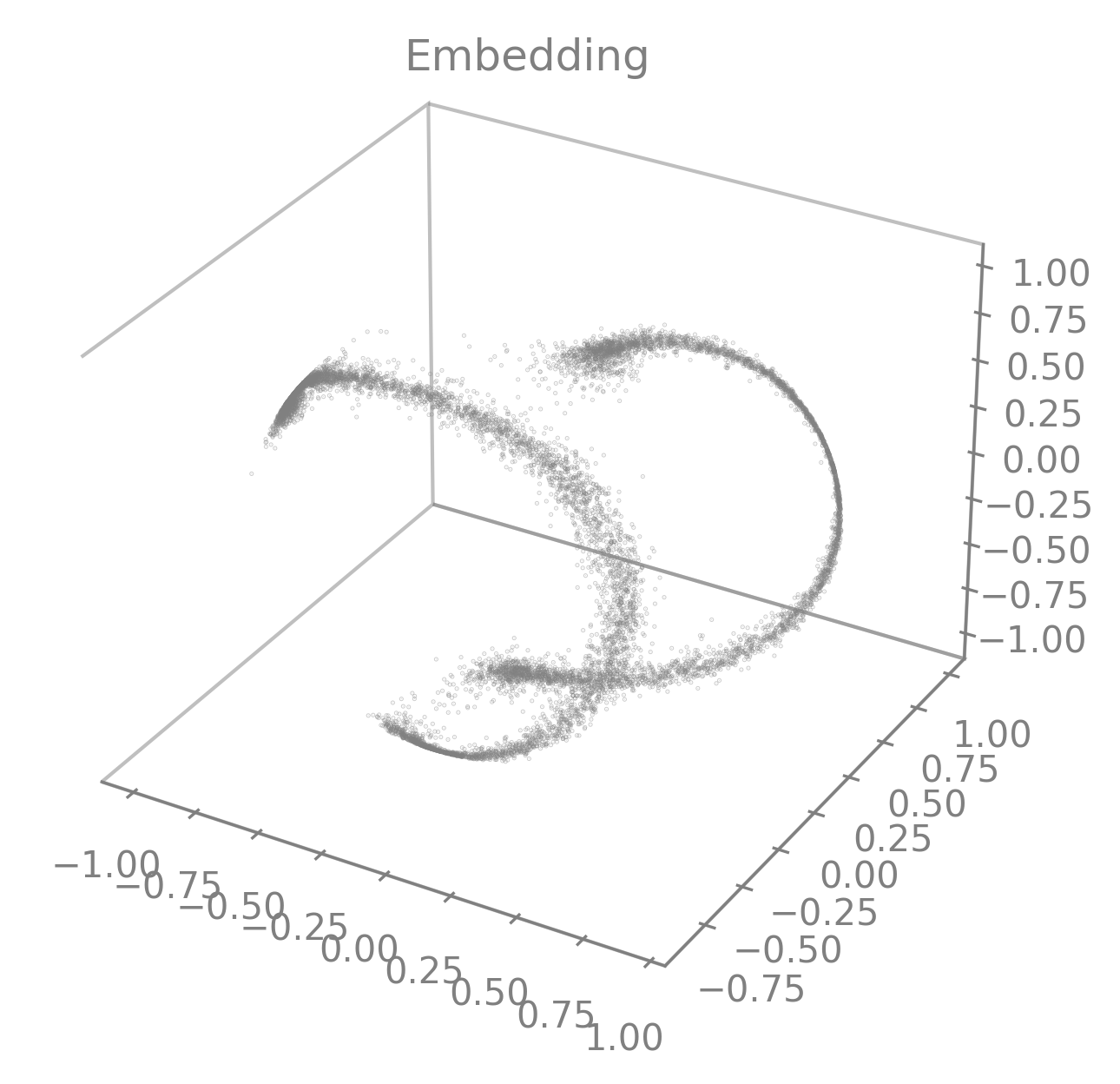
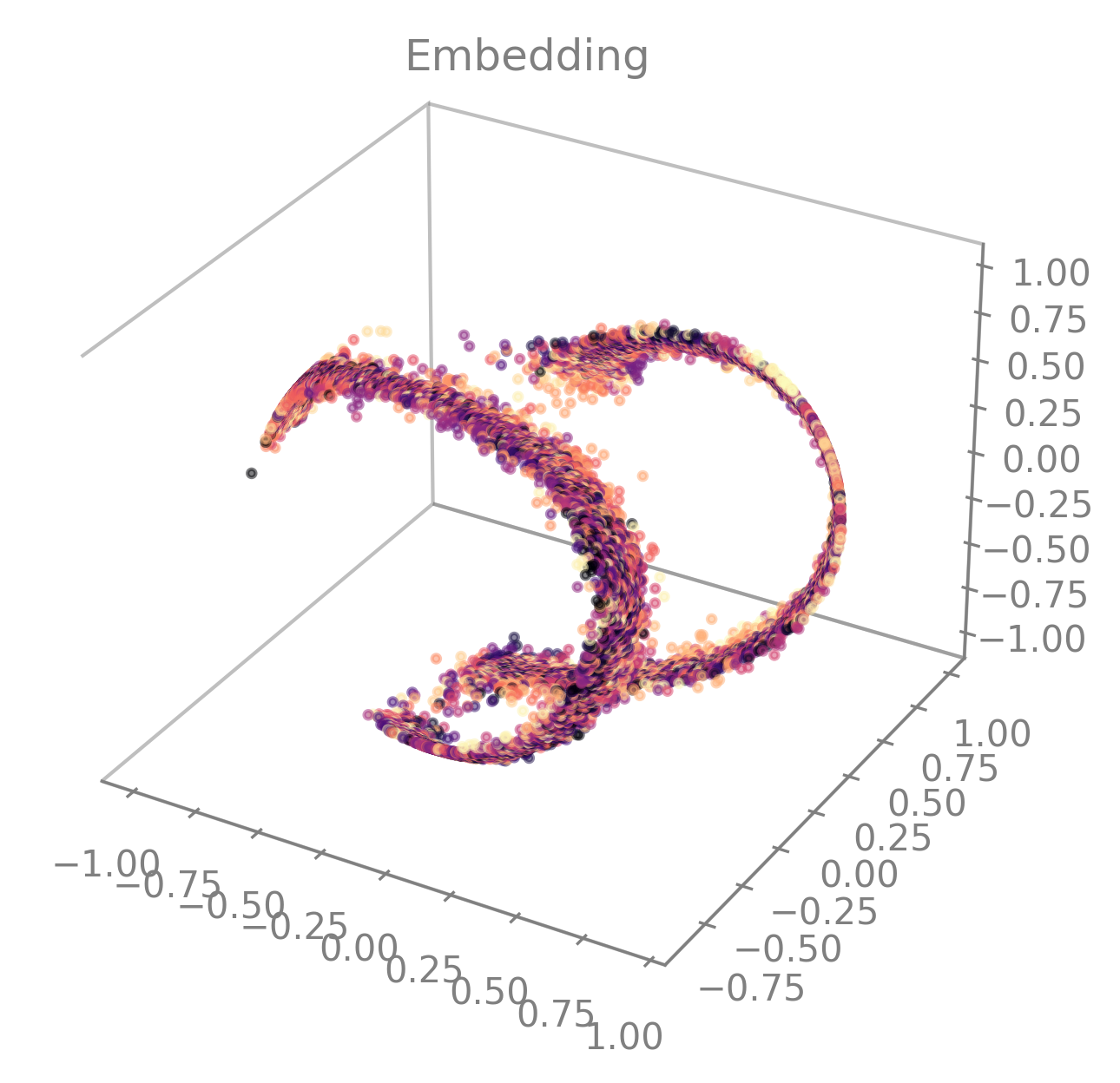
To get a 3D visualization of an embedding embedding, obtained using cebra.CEBRA.transform() (see above), you can use plot_embedding().

It takes a 2D matrix representing an embedding and returns a 3D scatter plot by taking the 3 first latents by default.

Note

If your embedding only has 2 dimensions, then the plot will automatically switch to a 2D mode. You can then use the function similarly.

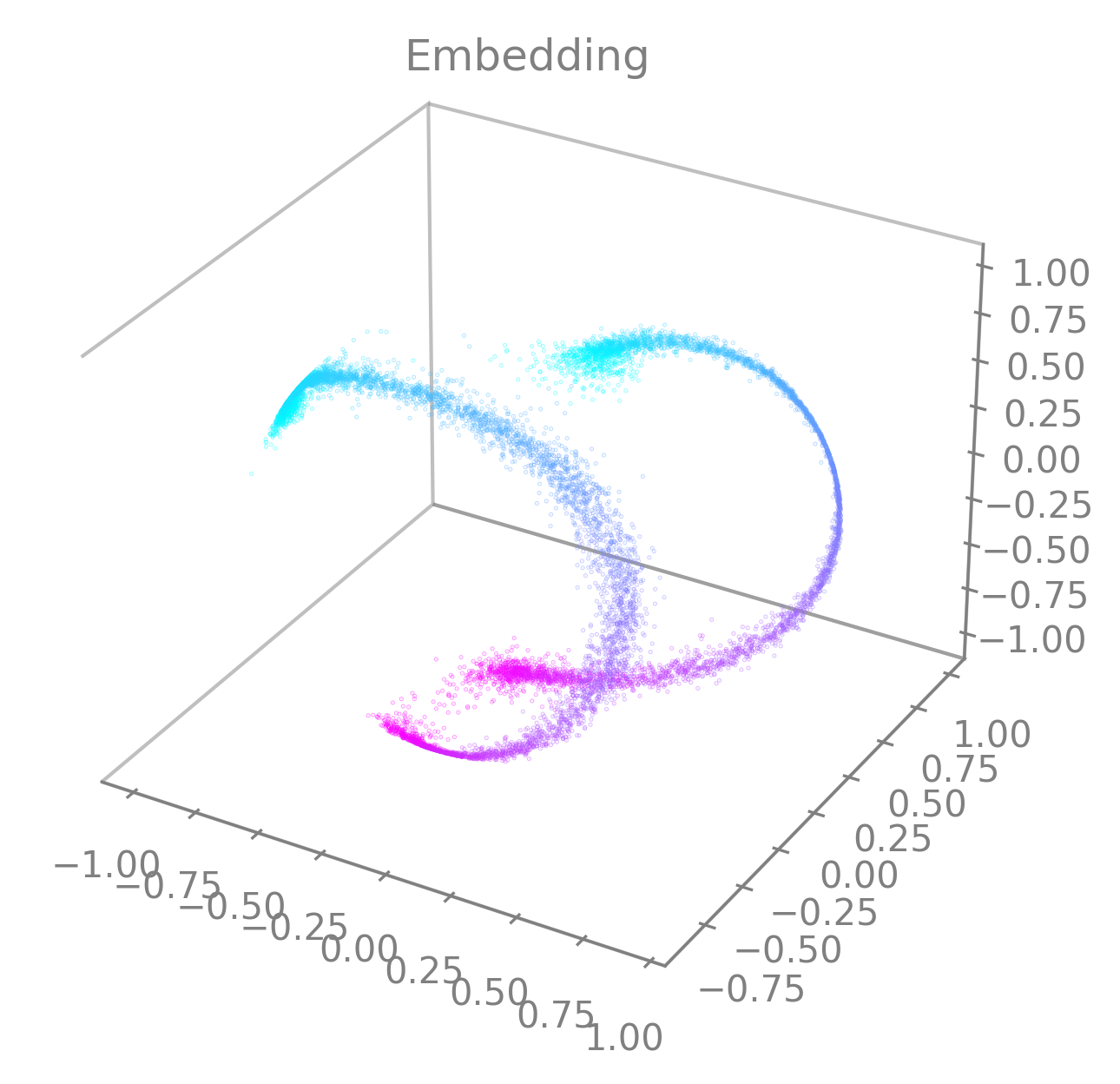
cebra.plot_embedding(embedding)

Note

Be aware that the latents are not visualized by rank of importance. Consequently if your embedding is initially larger than 3, a 3D-visualization taking the first 3 latents might not be a good representation of the most relevant features. Note that you can set the parameter idx_order to select the latents to display (see API).

🚀 Go further: personalize your embedding visualization

The function is a wrapper around matplotlib.pyplot.scatter() and consequently accepts all the parameters of that function (e.g., vmin, vmax, alpha, markersize, title, etc.) as parameters.

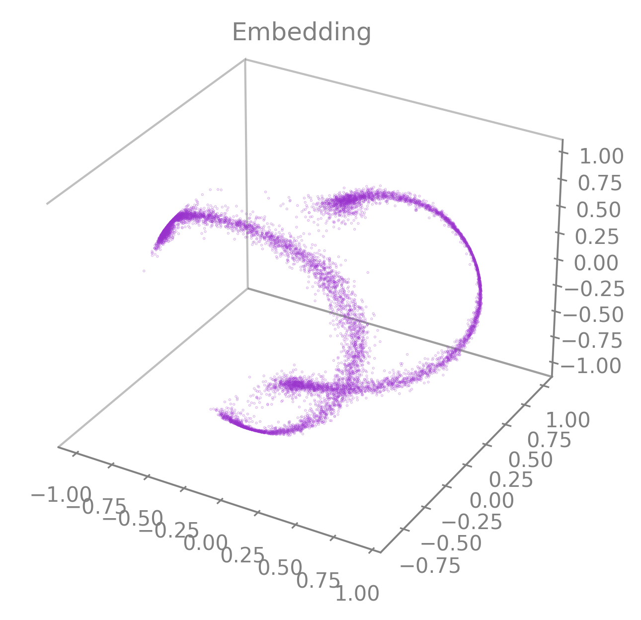
Regarding the color of the embedding, the default value is set to grey but can be customized using the parameter embedding_labels. There are 3 ways of doing it.

• By setting embedding_labels as a valid RGB(A) color (i.e., recognized by matplotlib, see Specifying colors for more details). You can use the following list of named colors as a good set of options already.

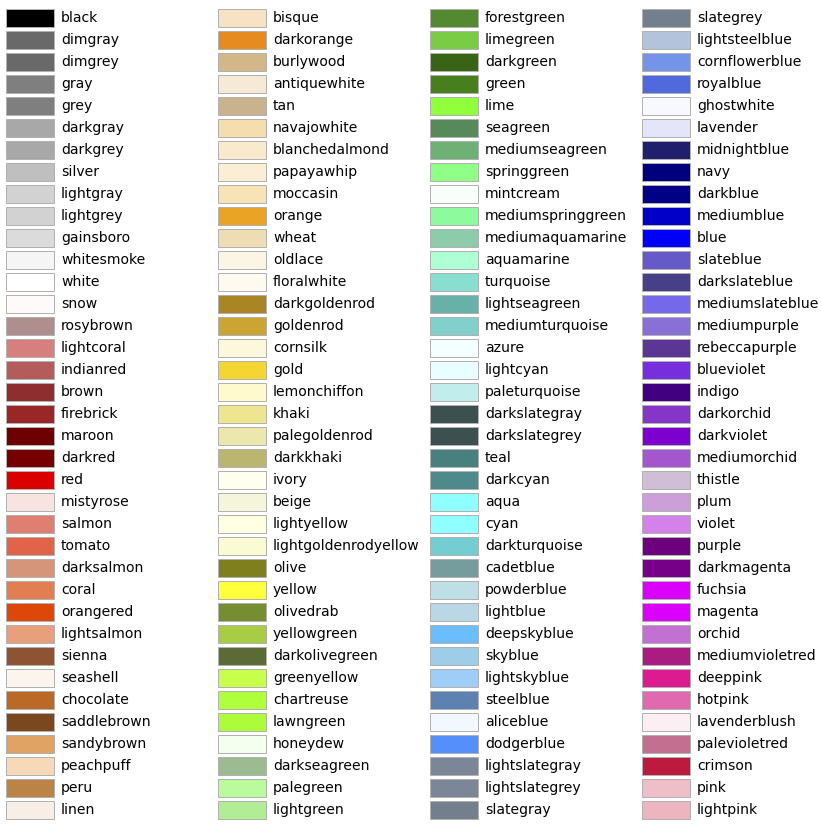
cebra.plot_embedding(embedding, embedding_labels="darkorchid")

• By setting embedding_labels to time. It will use the color map cmap to display the embedding based on temporality. By default, cmap=cool. You can customize it by setting it to a valid matplotlib.colors.Colormap (see Choosing Colormaps in Matplotlib for more information). You can also use our CEBRA-custom colormap by setting cmap="cebra".

CEBRA-custom colormap. You can use it by calling cmap="cebra" .

In the following example, you can also see how to change the size (markersize) or the transparency (alpha) of the markers.

cebra.plot_embedding(embedding, embedding_labels="time", cmap="magma", markersize=5, alpha=0.5)

• By setting embedding_labels as a vector of same size as the embedding to be mapped to colors, using cmap (see previous point for customization). The vector can consist of a discrete label or one of the auxiliary variables for example.

cebra.plot_embedding(embedding, embedding_labels=continuous_label[:, 0])

Note

embedding_labels must be uni-dimensional. Be sure to provide only one dimension of your auxiliary variables if you are using multi-dimensional continuous data for instance (e.g., only the x-coordinate of the position).

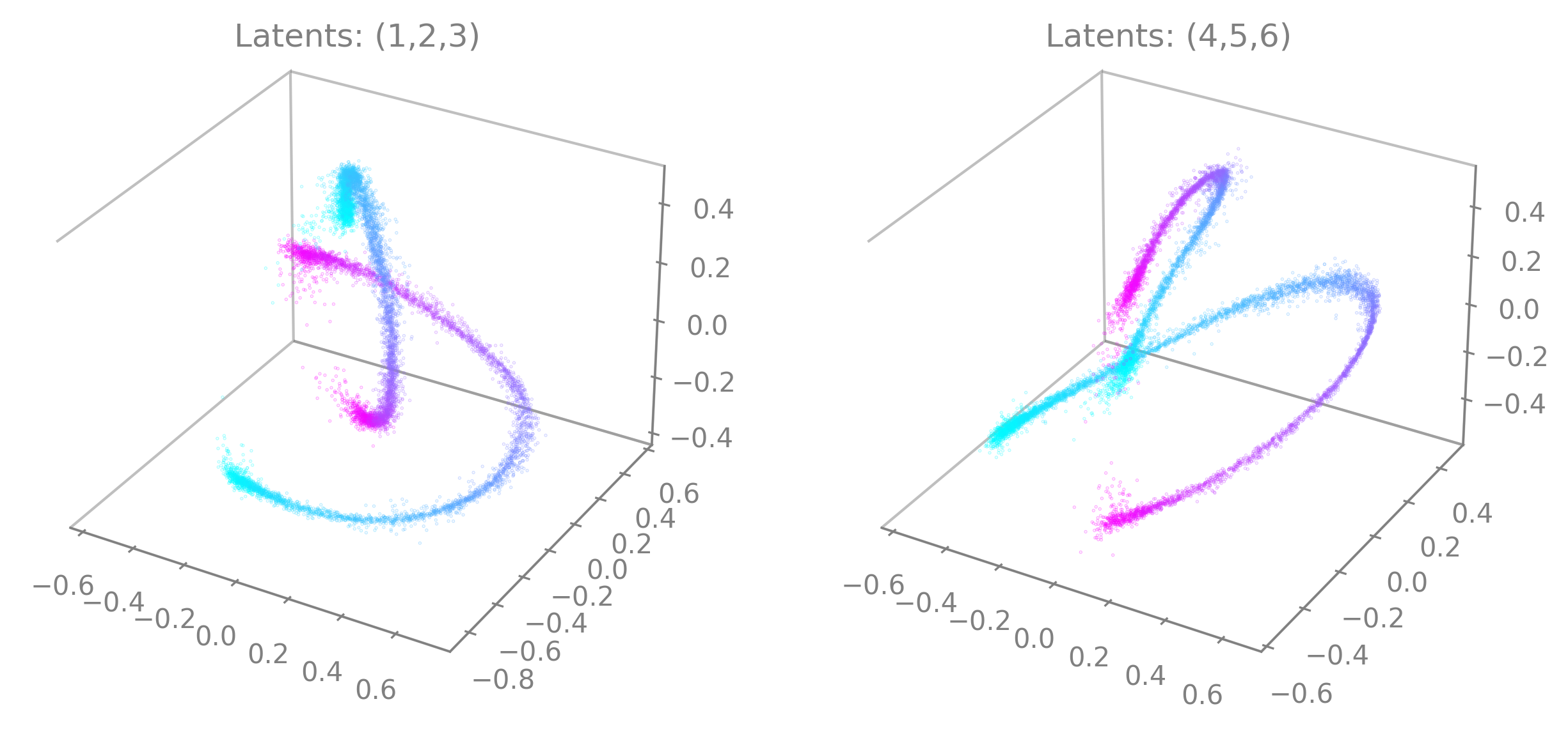
You can specify the latents to display by setting idx_order=(latent_num_1, latent_num_2, latent_num_3) with latent_num_* the latent indices of your choice. In the following example we trained a model with output_dimension==10 and we show embeddings when displaying latents (1, 2, 3) on the left and (4, 5, 6) on the right respectively. The code snippet also offers an example on how to combine multiple graphs and how to set a customized title (title). Note the parameter projection="3d" when adding a subplot to the figure.

import matplotlib.pyplot as plt
fig = plt.figure(figsize=(10,5))
ax1 = fig.add_subplot(121, projection="3d")
ax2 = fig.add_subplot(122, projection="3d")

ax1 = cebra.plot_embedding(embedding, embedding_labels=continuous_label[:,0], idx_order=(1,2,3), title="Latents: (1,2,3)", ax=ax1)
ax2 = cebra.plot_embedding(embedding, embedding_labels=continuous_label[:,0], idx_order=(4,5,6), title="Latents: (4,5,6)", ax=ax2)

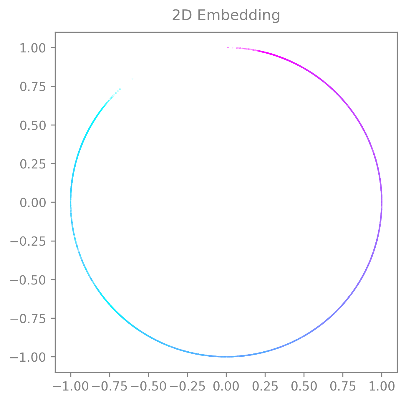
If your embedding only has 2 dimensions or if you only want to display 2 dimensions from it, you can use the same function. The plot will automatically switch to 2D. Then you can use the function as usual.

The plot will be 2D if:

• If your embedding only has 2 dimensions and you don’t specify the idx_order (then the default will be idx_order=(0,1))

• If your embedding is more than 2 dimensions but you specify the idx_order with only 2 dimensions.

cebra.plot_embedding(embedding, idx_order=(0,1), title="2D Embedding")

🚀 Look at the plot_embedding() API for more details on customization.

See API docs

cebra.plot_embedding(embedding, embedding_labels='grey', ax=None, idx_order=None, markersize=0.05, alpha=0.4, cmap='cool', title='Embedding', figsize=(5, 5), dpi=100, **kwargs)

Plot embedding in a 3D or 2D dimensional space.

If the embedding dimension is equal or higher to 3:

• If idx_order is not provided, the plot will be 3D by default.

• If idx_order is provided, and it has 3 dimensions, the plot will be 3D; if only 2 dimensions are provided, the plot will be 2D.

If the embedding dimension is equal to 2:

• If idx_order is not provided, the plot will be 2D by default.

• If idx_order is provided, and it has 3 dimensions, the plot will be 3D; if 2 dimensions are provided, the plot will be 2D.

This assumes that the dimensions provided to idx_order are within the range of the number of dimensions of the embedding (i.e., between 0 and cebra.CEBRA.output_dimension -1).

The function makes use of matplotlib.pyplot.scatter(), and parameters from that function can be provided as part of kwargs.

Parameters:

• embedding (Union[ndarray[tuple[int, ...], dtype[TypeVar(_ScalarType_co, bound= generic, covariant=True)]], Tensor]) – A matrix containing the feature representation computed with CEBRA.

• embedding_labels (Union[ndarray[tuple[int, ...], dtype[TypeVar(_ScalarType_co, bound= generic, covariant=True)]], Tensor, str, None]) –

  The labels used to map the data to color. It can be:

  • A vector that is the same sample size as the embedding, associating a value to each sample, either discrete or continuous.

  • A string, either time, which will color the embedding based on temporality, or a string that can be interpreted as an RGB(A) color, which will display the embedding uniformly with that color.

• ax (Optional[Axes]) – Optional axis to create the plot on.

• idx_order (Optional[Tuple[int]]) – A tuple (x, y, z) or (x, y) that maps a dimension in the data to a dimension in the 3D/2D embedding. The simplest form is (0, 1, 2) or (0, 1), but one might want to plot either those dimensions differently (e.g., (1, 0, 2)) or other dimensions from the feature representation (e.g., (2, 4, 5)).

• markersize (float) – The marker size.

• alpha (float) – The marker blending, between 0 (transparent) and 1 (opaque).

• cmap (str) – The Colormap instance or registered colormap name used to map scalar data to colors. It will be ignored if embedding_labels is set to a valid RGB(A).

• title (str) – The title on top of the embedding.

• figsize (Tuple[int]) – Figure width and height in inches.

• dpi (float) – Figure resolution.

• kwargs – Optional arguments to customize the plots. See matplotlib.pyplot.scatter() documentation for more details on which arguments to use.

Return type:

Axes

Returns:

The axis matplotlib.axes.Axes.axis() of the plot.

Example

>>> import cebra
>>> import numpy as np
>>> X = np.random.uniform(0, 1, (100, 50))
>>> y = np.random.uniform(0, 10, (100, 5))
>>> cebra_model = cebra.CEBRA(max_iterations=10)
>>> cebra_model.fit(X, y)
CEBRA(max_iterations=10)
>>> embedding = cebra_model.transform(X)
>>> ax = cebra.plot_embedding(embedding, embedding_labels='time')

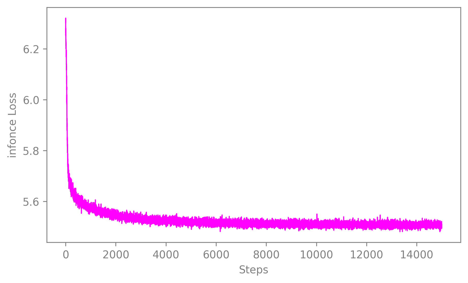
Displaying the training loss

Observing the training loss is of great importance. It allows you to assess that your model converged for instance or to compare models performances and fine-tune the parameters.

To visualize the loss evolution through training, you can use plot_loss().

It takes a CEBRA model and returns a 2D plot of the loss against the number of iterations. It can be used with default values as simply as this:

cebra.plot_loss(cebra_model)

🚀 The function is a wrapper around matplotlib.pyplot.plot() and consequently accepts all the parameters of that function (e.g., alpha, linewidth, title, color, etc.) as parameters.

See API docs

cebra.plot_loss(model, label=None, ax=None, color='magenta', linewidth=1, x_label=True, y_label=True, figsize=(7, 4), dpi=100, **kwargs)

Plot the evolution of loss during model training.

The function makes use of matplotlib.pyplot.plot() and parameters from that function can be provided as part of kwargs.

Parameters:

• model (CEBRA) – The (trained) CEBRA model.

• label (Union[str, int, float, None]) – The legend for the loss trace.

• ax (Optional[Axes]) – Optional axis to create the plot on.

• color (str) – Line color.

• linewidth (int) – Line width.

• x_label (bool) – A boolean that specifies if the x-axis label should be displayed.

• y_label (bool) – A boolean that specifies if the y-axis label should be displayed.

• figsize (tuple) – Figure width and height in inches.

• dpi (float) – Figure resolution.

• kwargs – Optional arguments to customize the plots. See matplotlib.pyplot.plot() documentation for more details on which arguments to use.

Example

>>> import cebra
>>> import numpy as np
>>> X = np.random.uniform(size=(100, 50))
>>> y = np.random.uniform(size=(100, 5))
>>> cebra_model = cebra.CEBRA(max_iterations=10)
>>> cebra_model.fit(X, y)
CEBRA(max_iterations=10)
>>> ax = cebra.plot_loss(cebra_model)

Return type:

Axes

Returns:

The axis matplotlib.axes.Axes.axis() of the plot.

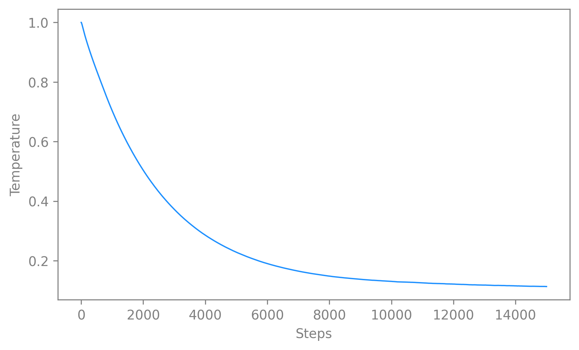
Displaying the temperature

temperature has the largest effect on the visualization of the embedding. Hence it might be interesting to check its evolution when temperature_mode=auto. We recommend only using auto if you have first explored the constant setting. If you use the auto mode, please always check the time evolution of the temperature over time alongside the loss curve.

To that extend, you can use the function plot_temperature().

It takes a CEBRA model and returns a 2D plot of the value of temperature against the number of iterations. It can be used with default values as simply as this:

cebra.plot_temperature(cebra_model)

🚀 The function is a wrapper around matplotlib.pyplot.plot() and consequently accepts all the parameters of that function (e.g., alpha, linewidth, title, color, etc.) as parameters.

See API docs

cebra.plot_temperature(model, ax=None, color='dodgerblue', linewidth=1, x_label=True, y_label=True, figsize=(7, 4), dpi=100, **kwargs)

Plot the evolution of the temperature hyperparameter during model training.

Note

It will vary only when using temperature_mode, else the temperature stays constant.

The function makes use of matplotlib.pyplot.plot() and parameters from that function can be provided as part of kwargs.

Parameters:

• model (CEBRA) – The (trained) CEBRA model.

• ax (Optional[Axes]) – Optional axis to create the plot on.

• color (str) – Line color.

• linewidth (int) – Line width.

• x_label (bool) – A boolean that specifies if the x-axis label should be displayed.

• y_label (bool) – A boolean that specifies if the y-axis label should be displayed.

• figsize (tuple) – Figure width and height in inches.

• dpi (float) – Figure resolution.

• kwargs – Optional arguments to customize the plots. See matplotlib.pyplot.plot() documentation for more details on which arguments to use.

Example

>>> import cebra
>>> import numpy as np
>>> X = np.random.uniform(0, 1, (100, 50))
>>> y = np.random.uniform(0, 10, (100, 5))
>>> cebra_model = cebra.CEBRA(max_iterations=10)
>>> cebra_model.fit(X, y)
CEBRA(max_iterations=10)
>>> ax = cebra.plot_temperature(cebra_model)

Return type:

Axes

Returns:

The axis matplotlib.axes.Axes.axis() of the plot.

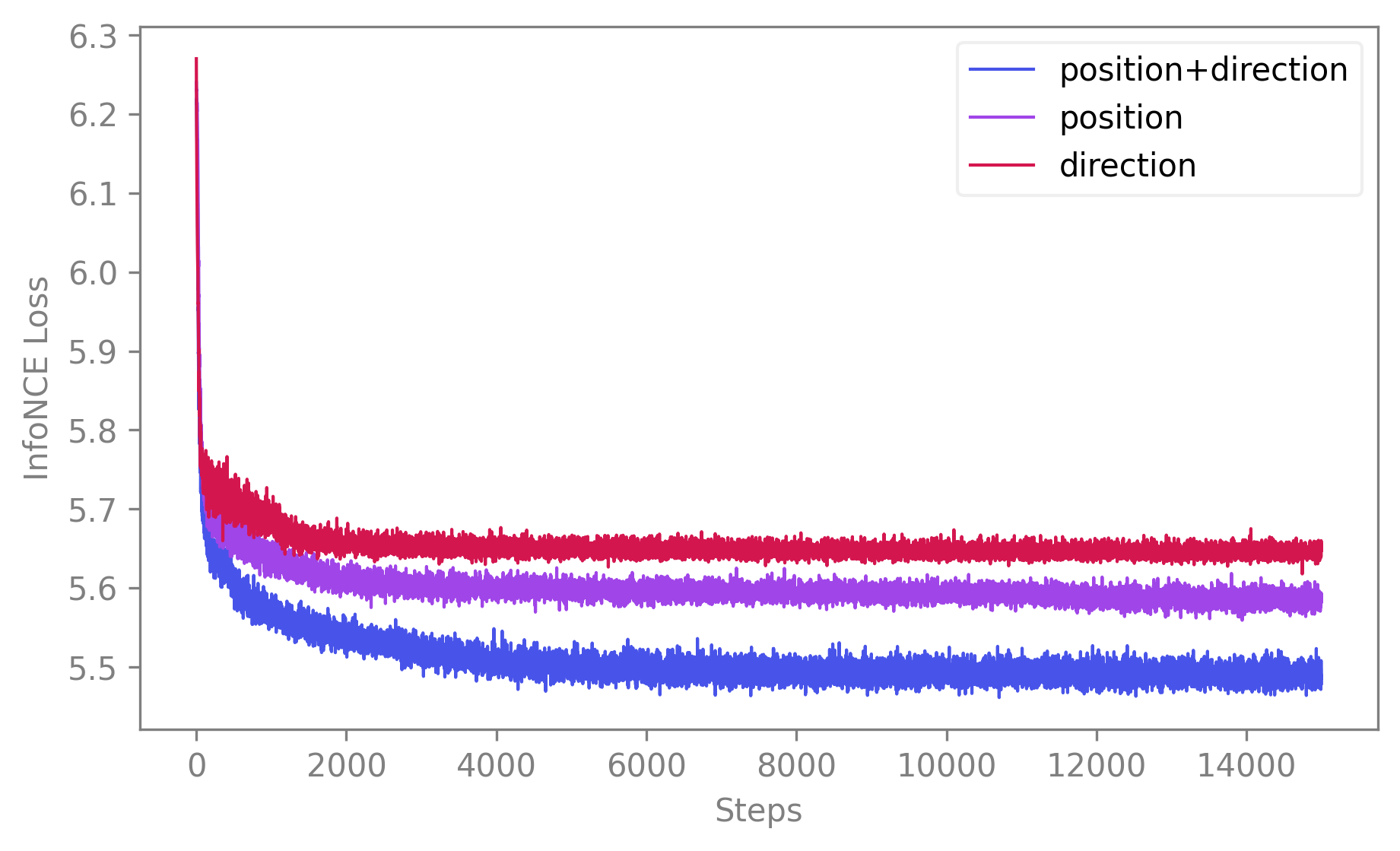
Comparing models

In order to select the most performant model, you might need to plot the training loss for a set of models on the same figure.

First, we create a list of fitted models to compare. Here we suppose we have a dataset with neural data available, as well as the position and the direction of the animal. We will show differences in performance when training with any combination of these variables.

cebra_posdir_model = CEBRA(model_architecture='offset10-model',
                batch_size=512,
                output_dimension=32,
                max_iterations=5,
                time_offsets=10)
cebra_posdir_model.fit(neural_data, continuous_label, discrete_label)

cebra_pos_model = CEBRA(model_architecture='offset10-model',
            batch_size=512,
            output_dimension=32,
            max_iterations=5,
            time_offsets=10)
cebra_pos_model.fit(neural_data, continuous_label)

cebra_dir_model = CEBRA(model_architecture='offset10-model',
            batch_size=512,
            output_dimension=32,
            max_iterations=5,
            time_offsets=10)
cebra_dir_model.fit(neural_data, discrete_label)

Then, you can compare their losses. To do that you can use compare_models(). It takes a list of CEBRA models and returns a 2D plot displaying their training losses. It can be used with default values as simply as this:

import cebra

# Labels to be used for the legend of the plot (optional)
labels = ["position+direction", "position", "direction"]

cebra.compare_models([cebra_posdir_model, cebra_pos_model, cebra_dir_model], labels)

🚀 The function is a wrapper around matplotlib.pyplot.plot() and consequently accepts all the parameters of that function (e.g., alpha, linewidth, title, color, etc.) as parameters. Note that however, if you want to differentiate the traces with a set of colors, you need to provide a colormap to the cmap parameter. If you want a unique color for all traces, you can provide a valid color to the color parameter that will override the cmap parameter. By default, color=None and cmap="cebra" our very special CEBRA-custom color map.

See API docs

cebra.compare_models(models, labels=None, ax=None, color=None, cmap='cebra', linewidth=1, x_label=True, y_label=True, figsize=(7, 4), dpi=100, **kwargs)

Plot the evolution of loss during model training.

The function makes use of matplotlib.pyplot.plot() and parameters from that function can be provided as part of kwargs.

Parameters:

• models (List[CEBRA]) – A list of trained CEBRA models.

• labels (Optional[List[str]]) – A list of labels, associated to each model to be used in the legend of the plot.

• ax (Optional[Axes]) – Optional axis to create the plot on.

• color (Optional[str]) – Line color. If not None, then all the traces for all models will be of the same color.

• cmap (str) – Color map from which to sample uniformly the quantitative list of colors for each trace. If color is different from then that parameter is ignored.

• linewidth (int) – Line width.

• x_label (bool) – A boolean that specifies if the x-axis label should be displayed.

• y_label (bool) – A boolean that specifies if the y-axis label should be displayed.

• figsize (tuple) – Figure width and height in inches.

• dpi (float) – Figure resolution.

• kwargs – Optional arguments to customize the plots. See matplotlib.pyplot.plot() documentation for more details on which arguments to use.

Example

>>> import cebra
>>> import numpy as np
>>> X = np.random.uniform(0, 1, (100, 50))
>>> y = np.random.uniform(0, 10, (100, 5))
>>> output_dimensions = [3, 8, 12, 32]
>>> models, labels = [], []
>>> for output_dimension in output_dimensions:
...     cebra_model = cebra.CEBRA(max_iterations=10,
...                               output_dimension=output_dimension)
...     cebra_model = cebra_model.fit(X, y)
...     models.append(cebra_model)
...     labels.append(f"Output dimension: {output_dimension}")
>>> ax = cebra.compare_models(models, labels)

Return type:

Axes

Returns:

The axis of the generated plot. If no ax argument was specified, it will be created by the function and returned here.

What else do to with your CEBRA model

As mentioned at the start of the guide, CEBRA is much more than a visualization tool. Here we present a (non-exhaustive) list of post-hoc analysis and investigations that we support with CEBRA. Happy hacking! 👩‍💻

Consistency across features

One of the major strengths of CEBRA is measuring consistency across embeddings. We demonstrate in Schneider, Lee, Mathis 2023, that consistent latents can be derived across animals (i.e., across CA1 recordings in rats), and even across recording modalities (i.e., from calcium imaging to electrophysiology recordings).

Thus, we provide the consistency_score() metrics to compute consistency across model runs or models computed on different datasets (i.e., subjects, sessions).

To use it, you have to set the between parameter to either datasets or runs. The main difference between the two modes is that for between-datasets comparisons you will provide labels to align the embeddings on. When using between-runs comparison, it supposes that the embeddings are already aligned. The simplest example being the model was run on the same dataset but it can also be for datasets that were recorded at the same time for example, i.e., neural activity in different brain regions, recorded during the same session.

Note

As consistency between CEBRA runs on the same dataset is demonstrated in Schneider, Lee, Mathis 2023 (consistent up to linear transformations), assessing consistency between different runs on the same dataset is a good way to reinsure you that you set your CEBRA model properly.

We first create the embeddings to compare: we use two different datasets of data and fit a CEBRA model three times on each.

n_runs = 3
dataset_ids = ["session1", "session2"]

cebra_model = CEBRA(model_architecture='offset10-model',
                batch_size=512,
                output_dimension=32,
                max_iterations=5,
                time_offsets=10)

embeddings_runs = []
embeddings_datasets, ids, labels = [], [], []
for i in range(n_runs):
    embeddings_runs.append(cebra_model.fit_transform(neural_session1, continuous_label1))

labels.append(continuous_label1[:, 0])
embeddings_datasets.append(embeddings_runs[-1])

embeddings_datasets.append(cebra_model.fit_transform(neural_session2, continuous_label2))
labels.append(continuous_label2[:, 0])

n_datasets = len(dataset_ids)

To get the consistency_score() on the set of embeddings that we just generated:

# Between-runs
scores_runs, pairs_runs, ids_runs = cebra.sklearn.metrics.consistency_score(embeddings=embeddings_runs,
                                                                            between="runs")
assert scores_runs.shape == (n_runs**2 - n_runs, )
assert pairs_runs.shape == (n_runs**2 - n_runs, 2)
assert ids_runs.shape == (n_runs, )

# Between-datasets, by aligning on the labels
(scores_datasets,
    pairs_datasets,
    ids_datasets) = cebra.sklearn.metrics.consistency_score(embeddings=embeddings_datasets,
                                                                labels=labels,
                                                                dataset_ids=dataset_ids,
                                                                between="datasets")
assert scores_datasets.shape == (n_datasets**2 - n_datasets, )
assert pairs_datasets.shape == (n_datasets**2 - n_datasets, 2)
assert ids_datasets.shape == (n_datasets, )

See API docs

cebra.sklearn.metrics.consistency_score(embeddings, between=None, labels=None, dataset_ids=None, num_discretization_bins=100)

Compute the consistency score between embeddings, either between runs or between datasets.

Parameters:

• embeddings (List[Union[ndarray[tuple[int, ...], dtype[TypeVar(_ScalarType_co, bound= generic, covariant=True)]], Tensor]]) – List of embedding matrices.

• labels (Optional[List[Union[ndarray[tuple[int, ...], dtype[TypeVar(_ScalarType_co, bound= generic, covariant=True)]], Tensor]]]) – List of labels corresponding to each embedding and to use for alignment between them. They are only required for a between-datasets comparison.

• dataset_ids (Optional[List[Union[int, str, float]]]) – List of dataset ID associated to each embedding. Multiple embeddings can be associated to the same dataset. In both modes (runs or datasets), if no dataset_ids is provided, then all the provided embeddings are compared one-to-one. Internally, the function will consider that the embeddings are all different runs from the same dataset for between-runs mode and on the contrary, that they are all computed on different dataset in the between-datasets mode.

• between (Optional[Literal[‘datasets’, ‘runs’]]) – A string describing the type of comparison to perform between the embeddings, either between all embeddings or between datasets or runs. Consistency between runs means the consistency between embeddings obtained from multiple models trained on the same dataset. Consistency between datasets means the consistency between embeddings obtained from models trained on different datasets, such as different animals, sessions, etc.

• num_discretization_bins (int) – Number of values for the digitalized common labels. The discretized labels are used for embedding alignment. Also see the n_bins argument in cebra.integrations.sklearn.helpers.align_embeddings for more information on how this parameter is used internally. This argument is only used if labels is not None, alignment between datasets is used (between = "datasets"), and the given labels are continuous and not already discrete.

Return type:

Tuple[ndarray[tuple[int, ...], dtype[TypeVar(_ScalarType_co, bound= generic, covariant=True)]], ndarray[tuple[int, ...], dtype[TypeVar(_ScalarType_co, bound= generic, covariant=True)]], ndarray[tuple[int, ...], dtype[TypeVar(_ScalarType_co, bound= generic, covariant=True)]]]

Returns:

The list of scores computed between the embeddings (first returns), the list of pairs corresponding to each computed score (second returns) and the list of id of the entities present in the comparison, either different datasets in the between-datasets comparison or runs in the between-runs comparison (third returns).

Example

>>> import cebra
>>> import numpy as np
>>> embedding1 = np.random.uniform(0, 1, (1000, 5))
>>> embedding2 = np.random.uniform(0, 1, (1000, 8))
>>> labels1 = np.random.uniform(0, 1, (1000, ))
>>> labels2 = np.random.uniform(0, 1, (1000, ))
>>> # Between-runs consistency
>>> scores, pairs, ids_runs = cebra.sklearn.metrics.consistency_score(embeddings=[embedding1, embedding2],
...                                                                   between="runs")
>>> # Between-datasets consistency, by aligning on the labels
>>> scores, pairs, ids_datasets = cebra.sklearn.metrics.consistency_score(embeddings=[embedding1, embedding2],
...                                                                   labels=[labels1, labels2],
...                                                                   dataset_ids=["achilles", "buddy"],
...                                                                   between="datasets")

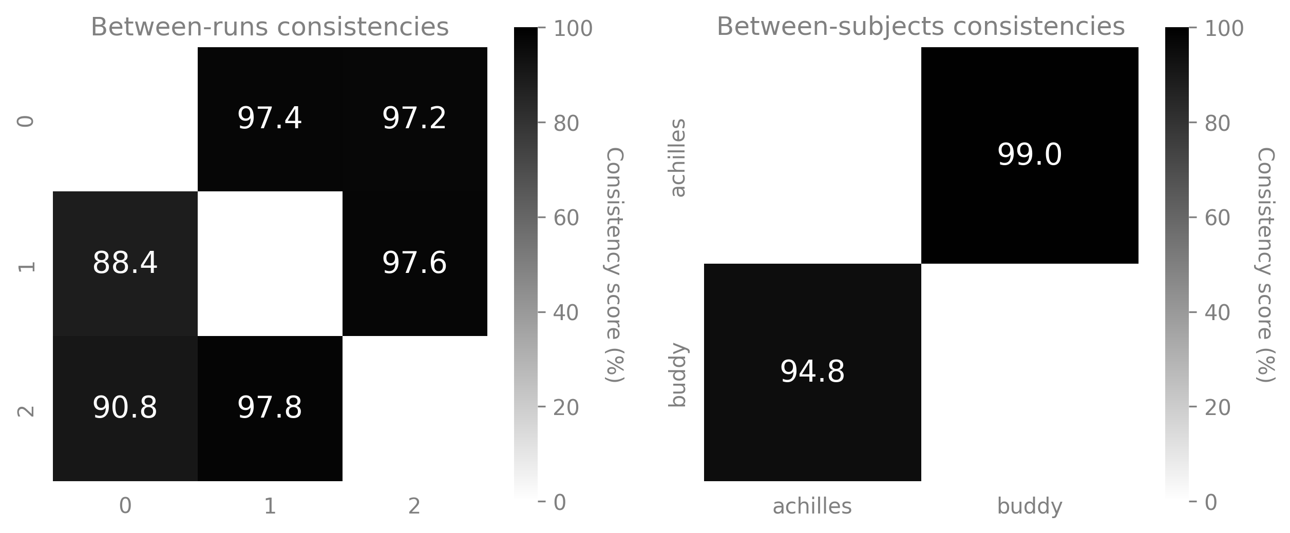
You can then display the resulting scores using plot_consistency().

fig = plt.figure(figsize=(10,4))

ax1 = fig.add_subplot(121)
ax2 = fig.add_subplot(122)

ax1 = cebra.plot_consistency(scores_runs, pairs_runs, ids_runs, vmin=0, vmax=100, ax=ax1, title="Between-runs consistencies")
ax2 = cebra.plot_consistency(scores_datasets, pairs_datasets, ids_runs, vmin=0, vmax=100, ax=ax2, title="Between-subjects consistencies")

🚀 This function is a wrapper around matplotlib.pyplot.imshow() and, similarly to the other plot functions we provide, it accepts all the parameters of that function (e.g., cmap, vmax, vmin, etc.) as parameters. Check the full API for more details.

See API docs

cebra.plot_consistency(scores, pairs=None, datasets=None, ax=None, cmap='binary', text_color='white', colorbar_label='Consistency score (%)', title=None, figsize=(5, 5), dpi=100, **kwargs)

Plot the consistency matrix from the consistency scores obtained with consistency_score().

To display the consistency map, datasets and pairs must be provided. The function is implemented so that it will first try to display the labels as if the scores were computed following a between-sujects comparison. If only one dataset is present or if the number of datasets doesn’t fit with the number of scores, then the function will display the labels as if the scores were computed following a between-runs comparison. If the number of pairs still doesn’t fit with that comparison, then an error is raised, asking the user to make sure that the formats of the scores, datasets and pairs are valid.

Tip

The safer way to use that function is to directly use as inputs the outputs from consistency_score().

The function makes use of matplotlib.pyplot.imshow() and parameters from that function can be provided as part of kwargs. For instance, we recommend that you bound the color bar using vmin and vmax. The scores are percentages between 0 and 100.

Parameters:

• scores (Union[ndarray[tuple[int, ...], dtype[TypeVar(_ScalarType_co, bound= generic, covariant=True)]], Tensor, list]) – List of consistency scores obtained by comparing a set of CEBRA embeddings using consistency_score().

• pairs (Union[list, ndarray[tuple[int, ...], dtype[TypeVar(_ScalarType_co, bound= generic, covariant=True)]], None]) – List of the pairs of datasets/runs whose embeddings were compared in scores.

• datasets (Union[list, ndarray[tuple[int, ...], dtype[TypeVar(_ScalarType_co, bound= generic, covariant=True)]], None]) – List of the datasets whose embeddings were compared in scores. Each dataset is present once only in the list.

• ax (Optional[Axes]) – Optional axis to create the plot on.

• cmap (str) – Color map to use to color the m

• text_color (str) – If None, then the scores values are not displayed, else, it corresponds to the color of the values displayed inside the grid.

• colorbar_label (Optional[str]) – If None, then the color bar is not shown, else, it defines the corresponding title.

• title (Optional[str]) – The title on top of the confusion matrix.

• figsize (Tuple[int]) – Figure width and height in inches.

• dpi (float) – Figure resolution.

• kwargs – Optional arguments to customize the plots. See matplotlib.pyplot.imshow() documentation for more details on which arguments to use.

Return type:

Axes

Returns:

The axis matplotlib.axes.Axes.axis() of the plot.

Example

>>> import cebra
>>> import numpy as np
>>> embedding1 = np.random.uniform(0, 1, (1000, 5))
>>> embedding2 = np.random.uniform(0, 1, (1000, 8))
>>> labels1 = np.random.uniform(0, 1, (1000, ))
>>> labels2 = np.random.uniform(0, 1, (1000, ))
>>> dataset_ids = ["achilles", "buddy"]
>>> # between-datasets consistency, by aligning on the labels
>>> scores, pairs, datasets = cebra.sklearn.metrics.consistency_score(
...     embeddings=[embedding1, embedding2],
...     labels=[labels1, labels2],
...     dataset_ids=dataset_ids,
...     between="datasets"
... )
>>> ax = cebra.plot_consistency(scores, pairs, datasets, vmin=0, vmax=100)

Embeddings comparison via the InfoNCE loss

Usage case 👩‍🔬

You can also compare how a new dataset compares to prior models. This can be useful when you have several groups of data and you want to see how a new session maps to the prior models. Then you will compute infonce_loss() of the new samples compared to other models.

How to use it

The performances of a given model on a dataset can be evaluated by using the infonce_loss() function. That metric corresponds to the loss over the data, obtained using the criterion on which the model was trained (by default, infonce). Hence, the smaller that metric is, the higher the model performances on a sample are, and so the better the fit to the positive samples is.

Note

As an indication, you can consider that a good trained CEBRA model should get a value for the InfoNCE loss smaller than ~6.1. If that is not the case, you might want to refer to the dedicated section Improve your model.

Here are examples on how you can use infonce_loss() on your data for both single-session and multi-session trained models.

# single-session
single_score = cebra.sklearn.metrics.infonce_loss(single_cebra_model,
                                                  neural_data,
                                                  continuous_label,
                                                  discrete_label,
                                                  num_batches=5)

# multi-session
multi_score = cebra.sklearn.metrics.infonce_loss(multi_cebra_model,
                                                 neural_session1,
                                                 continuous_label1,
                                                 session_id=0,
                                                 num_batches=5)

See API docs

cebra.sklearn.metrics.infonce_loss(cebra_model, X, *y, session_id=None, num_batches=500, correct_by_batchsize=False)

Compute the InfoNCE loss on a single session dataset on the model.

Parameters:

• cebra_model (CEBRA) – The model to use to compute the InfoNCE loss on the samples.

• X (Union[ndarray[tuple[int, ...], dtype[TypeVar(_ScalarType_co, bound= generic, covariant=True)]], Tensor]) – A 2D data matrix, corresponding to a single session recording.

• y – An arbitrary amount of continuous indices passed as 2D matrices, and up to one discrete index passed as a 1D array. Each index has to match the length of X.

• session_id (Optional[int]) – The session ID, an int between 0 and cebra.CEBRA.num_sessions for multisession, set to None for single session.

• num_batches (int) – The number of iterations to consider to evaluate the model on the new data. Higher values will give a more accurate estimate. Set it to at least 500 iterations.

• correct_by_batchsize (bool) – If True, the loss is corrected by the batch size.

Return type:

float

Returns:

The average InfoNCE loss estimated over num_batches batches from the data distribution.

Example

>>> import cebra
>>> import numpy as np
>>> neural_data = np.random.uniform(0, 1, (1000, 20))
>>> cebra_model = cebra.CEBRA(max_iterations=10)
>>> cebra_model.fit(neural_data)
CEBRA(max_iterations=10)
>>> loss = cebra.sklearn.metrics.infonce_loss(cebra_model,
...                                           neural_data,
...                                           num_batches=5)

Adapt the model to new data

In some cases, it can be useful to adapt your CEBRA model to a novel dataset, with a different number of features. For that, you can set adapt=True as a parameter of cebra.CEBRA.fit(). It will reset the first layer of the model so that the input dimension corresponds to the new features dimensions and retrain it for cebra.CEBRA.max_adapt_iterations. You can set that parameter cebra.CEBRA.max_adapt_iterations when initializing your cebra.CEBRA model.

Note

Adapting your CEBRA model to novel data is only implemented for single session training. Make sure that your model was trained on a single dataset.

# Fit your model once ...
single_cebra_model.fit(neural_session1)

# ... do something with it (embedding, visualization, saving) ...

# ... and adapt the model
cebra_model.fit(neural_session2, adapt=True)

Note

We recommend that you save your model, using cebra.CEBRA.save(), before adapting it to a different dataset. The adapted model will replace the previous model in cebra_model.state_dict_ so saving it beforehand allows you to keep the trained parameters for later. You can then load the model again, using cebra.CEBRA.load() whenever you need it.

See API docs

cebra.CEBRA.fit(self, X, *y, adapt=False, callback=None, callback_frequency=None)

Fit the estimator to the given dataset, either by initializing a new model or by adapting the existing trained model.

Note

Re-fitting a fitted model with fit() will reset the parameters and number of iterations. To continue fitting from the previous fit, partial_fit() must be used.

Tip

We recommend saving the model, using cebra.CEBRA.save(), before adapting it to a different dataset (setting adapt=True) as the adapted model will replace the previous model in cebra_model.state_dict_.

Parameters:

• X (Union[List[Iterable], Iterable]) – A 2D data matrix.

• y – An arbitrary amount of continuous indices passed as 2D matrices, and up to one discrete index passed as a 1D array. Each index has to match the length of X.

• adapt (bool) – If True, the estimator will be adapted to the given data. This parameter is of use only once the estimator has been fitted at least once (i.e., cebra.CEBRA.fit() has been called already). Note that it can be used on a fitted model that was saved and reloaded, using cebra.CEBRA.save() and cebra.CEBRA.load(). To adapt the model, the first layer of the model is reset so that it corresponds to the new features dimension. The parameters for all other layers are fixed and the first reinitialized layer is re-trained for cebra.CEBRA.max_adapt_iterations.

• callback (Optional[Callable[[int, Solver], None]]) – If a function is passed here with signature callback(num_steps, solver), the function will be regularly called at the specified callback_frequency.

• callback_frequency (Optional[int]) – Specify the number of iterations that need to pass before triggering the specified callback,

Return type:

CEBRA

Returns:

self, to allow chaining of operations.

Example

>>> import cebra
>>> import numpy as np
>>> import tempfile
>>> from pathlib import Path
>>> tmp_file = Path(tempfile.gettempdir(), 'cebra.pt')
>>> dataset =  np.random.uniform(0, 1, (1000, 20))
>>> dataset2 =  np.random.uniform(0, 1, (1000, 40))
>>> cebra_model = cebra.CEBRA(max_iterations=10)
>>> cebra_model.fit(dataset)
CEBRA(max_iterations=10)
>>> cebra_model.save(tmp_file)
>>> cebra_model.fit(dataset2, adapt=True)
CEBRA(max_iterations=10)
>>> tmp_file.unlink()

Decoding

The CEBRA latent embedding can be used for decoding analysis, meaning to investigate if a specific variable in the task can be decoded from the latent embeddings. Decoding using the embedding can be easily perform by mean of the decoders we implemented as part of CEBRA and following the scikit-learn API. We provide two decoders: KNNDecoder and L1LinearRegressor. Here is a simple usage of the KNNDecoder after using CEBRA-Time.

from sklearn.model_selection import train_test_split

# 1. Train a CEBRA-Time model on the whole dataset
cebra_model = cebra.CEBRA(max_iterations=10)
cebra_model.fit(neural_data)
embedding = cebra_model.transform(neural_data)

# 2. Split the embedding and label to decode into train/validation sets
(
     train_embedding,
     valid_embedding,
     train_discrete_label,
     valid_discrete_label,
) = train_test_split(embedding,
                     discrete_label,
                     test_size=0.3)

# 3. Train the decoder on the training set
decoder = cebra.KNNDecoder()
decoder.fit(train_embedding, train_discrete_label)

# 4. Get the score on the validation set
score = decoder.score(valid_embedding, valid_discrete_label)

# 5. Get the discrete labels predictions
prediction = decoder.predict(valid_embedding)

prediction contains the predictions of the decoder on the discrete labels.

Warning

Be careful to avoid double dipping when using the decoder. The previous example uses time contrastive learning. If you are using CEBRA-Behavior or CEBRA-Hybrid and you consequently use labels, you will have to split your original data from start as you don’t want decode labels from an embedding that is itself trained on those labels.

👉 Decoder example with CEBRA-Behavior

from sklearn.model_selection import train_test_split

# 1. Split your neural data and auxiliary variable
(
    train_data,
    valid_data,
    train_discrete_label,
    valid_discrete_label,
) = train_test_split(neural_data,
                     discrete_label,
                     test_size=0.2)

# 2. Train a CEBRA-Behavior model on training data only
cebra_model = cebra.CEBRA(max_iterations=10, batch_size=512)
cebra_model.fit(train_data, train_discrete_label)

# 3. Get embedding for training and validation data
train_embedding = cebra_model.transform(train_data)
valid_embedding = cebra_model.transform(valid_data)

# 4. Train the decoder on training embedding and labels
decoder = cebra.KNNDecoder()
decoder.fit(train_embedding, train_discrete_label)

# 5. Compute the score on validation embedding and labels
score = decoder.score(valid_embedding, valid_discrete_label)

See API docs

cebra.KNNDecoder.fit(self, X, y)

Fit the KNN decoder.

Parameters:

• X (Union[ndarray[tuple[int, ...], dtype[TypeVar(_ScalarType_co, bound= generic, covariant=True)]], Tensor]) – The data matrix.

• y (Union[ndarray[tuple[int, ...], dtype[TypeVar(_ScalarType_co, bound= generic, covariant=True)]], Tensor]) – A 1D array containing the targets.

Return type:

KNNDecoder

Returns:

self, to allow chaining of operations.

cebra.KNNDecoder.score(self, X, y)

Returns performances of the decoder instance on the provided data X.

Parameters:

• X (Union[ndarray[tuple[int, ...], dtype[TypeVar(_ScalarType_co, bound= generic, covariant=True)]], Tensor]) – A data matrix.

• y (Union[ndarray[tuple[int, ...], dtype[TypeVar(_ScalarType_co, bound= generic, covariant=True)]], Tensor]) – The true targets.

Return type:

Tuple[float, float, float]

Returns:

The R2 score on X.

Improve model performance

🧐 Below is a (non-exhaustive) list of actions you can try if your embedding looks different from what you were expecting.

1. Assess that your model converged. For that, observe if the training loss stabilizes itself around the end of the training or still seems to be decreasing. Refer to Visualize the training loss for more details on how to display the training loss.

2. Increase the number of iterations. It typically should be at least 10,000. On small datasets, it can make sense to stop training earlier to avoid overfitting effects.

3. Make sure the batch size is big enough. It should be at least 512.

4. Fine-tune the model’s hyperparameters, namely learning_rate, output_dimension, num_hidden_units and eventually temperature (by setting temperature_mode back to constant). Refer to Grid search for more details on performing hyperparameters tuning.

5. To note, you should still be mindful of performing train/validation splits and shuffle controls to avoid overfitting.

Quick Start: Scikit-learn API example

Putting all previous snippet examples together, we obtain the following pipeline.

import cebra
from numpy.random import uniform, randint
from sklearn.model_selection import train_test_split
import os
import tempfile
from pathlib import Path

# 1. Define a CEBRA model
cebra_model = cebra.CEBRA(
   model_architecture = "offset10-model",
   batch_size = 512,
   learning_rate = 1e-4,
   temperature_mode='constant',
   temperature = 0.1,
   max_iterations = 10, # TODO(user): to change to ~500-10000 depending on dataset size
   #max_adapt_iterations = 10, # TODO(user): use and to change to ~100-500 if adapting
   time_offsets = 10,
   output_dimension = 8,
   verbose = False
)

# 2. Load example data
neural_data = cebra.load_data(file="neural_data.npz", key="neural")
new_neural_data = cebra.load_data(file="neural_data.npz", key="new_neural")
continuous_label = cebra.load_data(file="auxiliary_behavior_data.h5", key="auxiliary_variables", columns=["continuous1", "continuous2", "continuous3"])
discrete_label = cebra.load_data(file="auxiliary_behavior_data.h5", key="auxiliary_variables", columns=["discrete"]).flatten()


assert neural_data.shape == (100, 3)
assert new_neural_data.shape == (100, 4)
assert discrete_label.shape == (100, )
assert continuous_label.shape == (100, 3)

# 3. Split data and labels into train/validation
from sklearn.model_selection import train_test_split

split_idx = int(0.8 * len(neural_data))
# suggestion: 5%-20% depending on your dataset size; note that this splits the
# into an early and late part, which might not be ideal for your data/experiment!
# As a more involved alternative, consider e.g. a nested time-series split.

train_data = neural_data[:split_idx]
valid_data = neural_data[split_idx:]

train_continuous_label = continuous_label[:split_idx]
valid_continuous_label = continuous_label[split_idx:]

train_discrete_label = discrete_label[:split_idx]
valid_discrete_label = discrete_label[split_idx:]

# 4. Fit the model
# time contrastive learning
cebra_model.fit(train_data)
# discrete behavior contrastive learning
cebra_model.fit(train_data, train_discrete_label)
# continuous behavior contrastive learning
cebra_model.fit(train_data, train_continuous_label)
# mixed behavior contrastive learning
cebra_model.fit(train_data, train_discrete_label, train_continuous_label)


# 5. Save the model
tmp_file = Path(tempfile.gettempdir(), 'cebra.pt')
cebra_model.save(tmp_file)

# 6. Load the model and compute an embedding
cebra_model = cebra.CEBRA.load(tmp_file)
train_embedding = cebra_model.transform(train_data)
valid_embedding = cebra_model.transform(valid_data)

assert train_embedding.shape == (80, 8) # TODO(user): change to split ratio & output dim
assert valid_embedding.shape == (20, 8) # TODO(user): change to split ratio & output dim

# 7. Evaluate the model performance (you can also check the train_data)
goodness_of_fit = cebra.sklearn.metrics.goodness_of_fit_score(cebra_model,
                                                     valid_data,
                                                     valid_discrete_label,
                                                     valid_continuous_label)

# 8. Adapt the model to a new session
cebra_model.fit(new_neural_data, adapt = True)

# 9. Decode discrete labels behavior from the embedding
decoder = cebra.KNNDecoder()
decoder.fit(train_embedding, train_discrete_label)
prediction = decoder.predict(valid_embedding)
assert prediction.shape == (20,)

👉 For further guidance on different/customized applications of CEBRA on your own data, refer to the examples/ folder or to the full documentation folder docs/.

Quick Start: Torch API example

🚀 You have special custom data analysis needs or want more features? We invite you to use the torch-API interface.

Refer to the Demos tab for a demo notebook using the torch-API: https://cebra.ai/docs/demo_notebooks/Demo_Allen.html.

Single- and multi-session training could be launched using the following bash command.

$ PYTHONPATH=. python examples/train.py [customized arguments]

Below is the documentation on the available arguments.

$ PYTHONPATH=. python examples/train.py --help
usage: train.py [-h] [--data <dataclasses._MISSING_TYPE object at 0x7f2eeb13f070>] [--variant single-session]
                [--logdir /logs/single-rat-hippocampus-behavior/] [--loss-distance cosine] [--temperature 1]
                [--time-offset 10] [--conditional time_delta] [--num-steps 1000] [--learning-rate 0.0003]
                [--model offset10-model] [--batch-size 512] [--num-hidden-units 32] [--num-output 8] [--device cpu]
                [--tqdm False] [--save-frequency SAVE_FREQUENCY] [--valid-frequency 100] [--train-ratio 0.8]
                [--valid-ratio 0.1] [--share-model]

CEBRA Demo

options:
-h, --help            show this help message and exit
--data <dataclasses._MISSING_TYPE object at 0x7f2eeb13f070>
                        The dataset to run CEBRA on. Standard datasets are available in cebra.datasets. Your own datasets can
                        be created by subclassing cebra.data.Dataset and registering the dataset using the
                        ``@cebra.datasets.register`` decorator.
--variant single-session
                        The CEBRA variant to run.
--logdir /logs/single-rat-hippocampus-behavior/
                        Model log directory. This should be either a new empty directory, or a pre-existing directory
                        containing a trained CEBRA model.
--loss-distance cosine
                        Distance type to use in calculating loss
--temperature 1       Temperature for InfoNCE loss
--time-offset 10      Distance (in time) between positive pairs. The interpretation of this parameter depends on the chosen
                        conditional distribution, but generally a higher time offset increases the difficulty of the learning
                        task, and (in a certain range) improves the quality of the representation. The time offset would
                        typically be larger than the specified receptive field of the model.
--conditional time_delta
                        Type of conditional distribution. Valid standard methods are "time_delta" and "time", and more
                        methods can be added to the ``cebra.data`` registry.
--num-steps 1000      Number of total training steps. Number of total training steps. Note that training duration of CEBRA
                        is independent of the dataset size. The total training examples seen will amount to ``num-steps x
                        batch-size``, irrespective of dataset size.
--learning-rate 0.0003
                        Learning rate for Adam optimizer.
--model offset10-model
                        Model architecture. Available options are 'offset10-model', 'offset5-model' and 'offset1-model'.
--batch-size 512      Total batch size for each training step.
--num-hidden-units 32
                        Number of hidden units.
--num-output 8        Dimension of output embedding
--device cpu          Device for training. Options: cpu/cuda
--tqdm False          Activate tqdm for logging during the training
--save-frequency SAVE_FREQUENCY
                        Interval of saving intermediate model
--valid-frequency 100
                        Interval of validation in training
--train-ratio 0.8     Ratio of train dataset. The remaining will be used for valid and test split.
--valid-ratio 0.1     Ratio of validation set after the train data split. The remaining will be test split
--share-model

Model training using the Torch API

The scikit-learn API provides parametrization to many common use cases. The Torch API however allows for more flexibility and customization, for e.g. sampling, criterions, and data loaders.

In this minimal example we show how to initialize a CEBRA model using the Torch API. Here the cebra.data.single_session.DiscreteDataLoader gets initialized which also allows the prior to be directly parametrized.

👉 For an example notebook using the Torch API check out the Decoding movie features from (V1) visual cortex.

import numpy as np
import cebra.datasets
import torch

if torch.cuda.is_available():
    device = "cuda"
else:
    device = "cpu"

neural_data = cebra.load_data(file="neural_data.npz", key="neural")

discrete_label = cebra.load_data(
    file="auxiliary_behavior_data.h5", key="auxiliary_variables", columns=["discrete"],
)

# 1. Define a CEBRA-ready dataset
input_data = cebra.data.TensorDataset(
    torch.from_numpy(neural_data).type(torch.FloatTensor),
    discrete=torch.from_numpy(np.array(discrete_label[:, 0])).type(torch.LongTensor),
).to(device)

# 2. Define a CEBRA model
neural_model = cebra.models.init(
    name="offset10-model",
    num_neurons=input_data.input_dimension,
    num_units=32,
    num_output=2,
).to(device)

input_data.configure_for(neural_model)

# 3. Define the Loss Function Criterion and Optimizer
crit = cebra.models.criterions.LearnableCosineInfoNCE(
    temperature=1,
).to(device)

opt = torch.optim.Adam(
    list(neural_model.parameters()) + list(crit.parameters()),
    lr=0.001,
    weight_decay=0,
)

# 4. Initialize the CEBRA model
solver = cebra.solver.init(
    name="single-session",
    model=neural_model,
    criterion=crit,
    optimizer=opt,
    tqdm_on=True,
).to(device)

# 5. Define Data Loader
loader = cebra.data.single_session.DiscreteDataLoader(
    dataset=input_data, num_steps=10, batch_size=200, prior="uniform"
)

# 6. Fit Model
solver.fit(loader=loader)

# 7. Transform Embedding
train_batches = np.lib.stride_tricks.sliding_window_view(
    neural_data, neural_model.get_offset().__len__(), axis=0
)

x_train_emb = solver.transform(
    torch.from_numpy(train_batches[:]).type(torch.FloatTensor).to(device)
).to(device)

# 8. Plot Embedding
cebra.plot_embedding(
    x_train_emb.cpu(),
    discrete_label[neural_model.get_offset().__len__() - 1 :, 0],
    markersize=10,
)