You can download and run the notebook locally or run it with Google Colaboratory:
![]()
Encoding of space, hippocampus (CA1)#
In this notebook, we show how to:
use CEBRA on the hippocampus data.
use CEBRA with our scikit-learn API.
use the infoNCE loss for supervised and self-supervised learning within CEBRA.
More specifically, this is a notebook demonstrating the information presented in Hypothesis-driven analysis, Consistency, Decoding and Topological Data Analysis into a single demo notebook. We recommend that you go through those individual notebooks for more informtion.
[ ]:
!pip install --pre 'cebra[datasets, integrations]'

# later in the notebook we are going to do some topological data analysis, and we grab some precomputed results:
!pip install ripser
!pip install git+https://github.com/ctralie/DREiMac.git@cdd6d02ba53c3597a931db9da478fd198d6ed00f
!wget https://github.com/AdaptiveMotorControlLab/CEBRA-demos/raw/main/rat_demo_example_output.h5
[2]:
import sys

import numpy as np
import pandas as pd
import matplotlib.pyplot as plt
import joblib as jl
import cebra.datasets
from cebra import CEBRA

from matplotlib.collections import LineCollection
import pandas as pd
Load the data:#
The data will be automatically downloaded into a
/datafolder.
[3]:
#1. Load example data
%mkdir data
hippocampus_pos = cebra.datasets.init('rat-hippocampus-single-achilles')
100%|██████████| 10.0M/10.0M [00:01<00:00, 5.17MB/s]
Download complete. Dataset saved in 'data/rat_hippocampus/achilles.jl'
Visualize the data:#
[4]:
fig = plt.figure(figsize=(9,3), dpi=150)
plt.subplots_adjust(wspace = 0.3)
ax = plt.subplot(121)
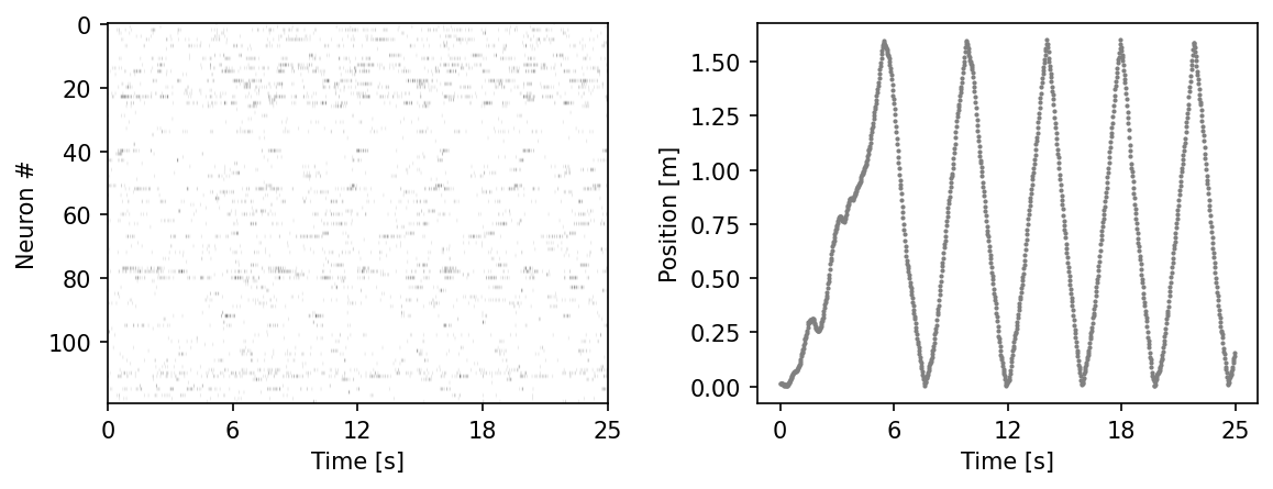
ax.imshow(hippocampus_pos.neural.numpy()[:1000].T, aspect = 'auto', cmap = 'gray_r')
plt.ylabel('Neuron #')
plt.xlabel('Time [s]')
plt.xticks(np.linspace(0, 1000, 5), np.linspace(0, 0.025*1000, 5, dtype = int))
ax2 = plt.subplot(122)
ax2.scatter(np.arange(1000), hippocampus_pos.continuous_index[:1000,0], c = 'gray', s=1)
plt.ylabel('Position [m]')
plt.xlabel('Time [s]')
plt.xticks(np.linspace(0, 1000, 5), np.linspace(0, 0.025*1000, 5, dtype = int))
plt.show()
CEBRA-Behavior: Train a model with 3D output that uses positional information (position + direction).#
Please be aware this is JUST a demo notebook; for details on reproducing our paper results, see the paper.
Please see our user docs for our suggestions on properly using CEBRA for experiments.
Setting conditional = ‘time_delta’ means we will use CEBRA-Behavior mode and use auxiliary behavior variable for the model training.
For a quick CPU run-time demo, you can drop
max_iterationsto 100-500; otherwise, set to ~5-10000 on a GPU for a reasonable demo.For a demonstration relating to Figure 2, we use output dimension 3 for the infoNCE loss.
[5]:
max_iterations = 5000
[6]:
#2. Define the model
cebra_posdir3_model = CEBRA(model_architecture='offset10-model',
                        batch_size=512,
                        learning_rate=3e-4,
                        temperature=1,
                        output_dimension=3,
                        max_iterations=max_iterations,
                        distance='cosine',
                        conditional='time_delta',
                        device='cuda_if_available',
                        verbose=True,
                        time_offsets=10)
Attention: Here we split the data for train/validation into 80/20. Note, the behavior might not be the same in the first 80% vs. last 20%, therefore, we recommend cross validating with different splitting strategies when when you use this feature! Read more at sklearn.
[7]:
# 3. Split data and labels
from sklearn.model_selection import train_test_split
split_idx = int(0.8 * len(hippocampus_pos.neural)) #suggest: 5%-20% depending on your dataset size

train_data = hippocampus_pos.neural[:split_idx]
valid_data = hippocampus_pos.neural[split_idx:]

train_continuous_label = hippocampus_pos.continuous_index.numpy()[:split_idx]
valid_continuous_label = hippocampus_pos.continuous_index.numpy()[split_idx:]
We train the model with neural data and the behavior variable including position and direction.#
with a V100 GPU, 5K iterations should take less then 2 min.
[8]:
# 4. Fit the model
cebra_posdir3_model.fit(train_data, train_continuous_label)
pos: -0.8875 neg: 6.4205 total: 5.5330 temperature: 1.0000: 100%|██████████| 5000/5000 [00:47<00:00, 104.60it/s]
[8]:
CEBRA(batch_size=512, conditional='time_delta', max_iterations=5000,
      model_architecture='offset10-model', output_dimension=3, temperature=1,
      time_offsets=10, verbose=True)
In a Jupyter environment, please rerun this cell to show the HTML representation or trust the notebook. On GitHub, the HTML representation is unable to render, please try loading this page with nbviewer.org.
CEBRA(batch_size=512, conditional='time_delta', max_iterations=5000,
      model_architecture='offset10-model', output_dimension=3, temperature=1,
      time_offsets=10, verbose=True)
[9]:
# 5. Save the model
import os
import tempfile
from pathlib import Path
tmp_file = Path(tempfile.gettempdir(), 'cebra.pt')
cebra_posdir3_model.save(tmp_file)
[10]:
# 6. Load the model and compute an embedding
cebra_posdir3_model = cebra.CEBRA.load(tmp_file)
train_embedding = cebra_posdir3_model.transform(train_data)
valid_embedding = cebra_posdir3_model.transform(valid_data)
[11]:
# 7. Evaluate the model performance on the train set
goodness_of_fit = cebra.sklearn.metrics.infonce_loss(cebra_posdir3_model,
                                                     train_data,
                                                     train_continuous_label,
                                                     num_batches=5)
print(" goodness of fit - train:",goodness_of_fit)
100%|██████████| 5/5 [00:00<00:00, 236.12it/s]
goodness of fit - train: 5.533586883544922
Visualize the embedding#
Note, CEBRA’s strength is quantitative measures of the resulting embedding with goodness of fit and consistency (comparisions across models, etc). But, it is useful to visualize the data for a qualitative assessment.
If it’s collapsed or points are uniformly scattered across the sphere, either your label is not well represented in your data, or you need to adjust your model.
[12]:
import cebra.integrations.plotly

fig = cebra.integrations.plotly.plot_embedding_interactive(train_embedding,
                                                           embedding_labels=train_continuous_label[:,0],
                                                           title = "CEBRA-Behavior Train",
                                                           markersize=2,
                                                           cmap = "rainbow")
fig.show()
<Figure size 500x500 with 0 Axes>
[13]:
import cebra.integrations.plotly

fig = cebra.integrations.plotly.plot_embedding_interactive(valid_embedding,
                                                           embedding_labels=valid_continuous_label[:,0],
                                                           title = "CEBRA-Behavior-validation",
                                                           markersize=2,
                                                           cmap = "rainbow")
fig.show()
<Figure size 500x500 with 0 Axes>
Shuffle Control#
beyond train/validation splits we can compare a shuffle embedding with the same hyperparameters
[14]:
### Shuffle the behavior variable and use it for training
hippocampus_shuffled_posdir = np.random.permutation(hippocampus_pos.continuous_index.numpy())
[15]:
# Shuffle: Split data and labels

split_idx = int(0.8 * len(hippocampus_shuffled_posdir)) #suggest: 5%-20% depending on your dataset size

shuffle_train_data = hippocampus_pos.neural[:split_idx]
shuffle_valid_data = hippocampus_pos.neural[split_idx:]

train_continuous_label = hippocampus_shuffled_posdir[:split_idx]
valid_continuous_label = hippocampus_shuffled_posdir[split_idx:]
[16]:
cebra_posdir3_model.fit(shuffle_train_data, train_continuous_label)
pos: -0.7006 neg: 6.8378 total: 6.1371 temperature: 1.0000: 100%|██████████| 5000/5000 [00:48<00:00, 104.09it/s]
[16]:
CEBRA(batch_size=512, conditional='time_delta', max_iterations=5000,
      model_architecture='offset10-model', output_dimension=3, temperature=1,
      time_offsets=10, verbose=True)
In a Jupyter environment, please rerun this cell to show the HTML representation or trust the notebook. On GitHub, the HTML representation is unable to render, please try loading this page with nbviewer.org.
CEBRA(batch_size=512, conditional='time_delta', max_iterations=5000,
      model_architecture='offset10-model', output_dimension=3, temperature=1,
      time_offsets=10, verbose=True)
[17]:
shuffle_train_embedding = cebra_posdir3_model.transform(shuffle_train_data)
shuffle_valid_embedding = cebra_posdir3_model.transform(shuffle_valid_data)
[18]:
# Evaluate the model performance on the train shuffle set
goodness_of_fit = cebra.sklearn.metrics.infonce_loss(cebra_posdir3_model,
                                                     shuffle_train_data,
                                                     train_continuous_label,
                                                     num_batches=5)
print(" goodness of fit - shuffle train:",goodness_of_fit)
100%|██████████| 5/5 [00:00<00:00, 235.95it/s]
goodness of fit - shuffle train: 6.163306331634521
[19]:
fig = cebra.integrations.plotly.plot_embedding_interactive(shuffle_train_embedding,
                                                           embedding_labels=train_continuous_label[:,0],
                                                           title = "CEBRA-Behavior Shuffle Train",
                                                           markersize=2,
                                                           cmap = "rainbow")
fig.show()
<Figure size 500x500 with 0 Axes>
[20]:
fig = cebra.integrations.plotly.plot_embedding_interactive(shuffle_valid_embedding,
                                                           embedding_labels=valid_continuous_label[:,0],
                                                           title = "CEBRA-Behavior Shuffle Validation",
                                                           markersize=2,
                                                           cmap = "rainbow")
fig.show()
<Figure size 500x500 with 0 Axes>
Using the full data#
Now that we have checked our parameters are not causing overfitting, we will train on the full dataset so we can make comparisons below.
[21]:
cebra_posdir3_model.fit(hippocampus_pos.neural, hippocampus_pos.continuous_index.numpy())
cebra_posdir3 = cebra_posdir3_model.transform(hippocampus_pos.neural)
pos: -0.9002 neg: 6.4140 total: 5.5138 temperature: 1.0000: 100%|██████████| 5000/5000 [00:49<00:00, 101.55it/s]
[22]:
fig = cebra.integrations.plotly.plot_embedding_interactive(cebra_posdir3, embedding_labels=hippocampus_pos.continuous_index[:,0], title = "CEBRA-Behavior", markersize=2, cmap = "rainbow")
fig.show()
<Figure size 500x500 with 0 Axes>
CEBRA-Shuffled Behavior: Train a control model with shuffled neural data.#
The model specification is the same as the CEBRA-Behavior above.
Note, here we do not demonstrate the train/val split.
[23]:
cebra_posdir_shuffled3_model = CEBRA(model_architecture='offset10-model',
                        batch_size=512,
                        learning_rate=3e-4,
                        temperature=1,
                        output_dimension=3,
                        max_iterations=max_iterations,
                        distance='cosine',
                        conditional='time_delta',
                        device='cuda_if_available',
                        verbose=True,
                        time_offsets=10)
Now we train the model with shuffled behavior variable.
[24]:
### Shuffle the behavior variable and use it for training
hippocampus_shuffled_posdir = np.random.permutation(hippocampus_pos.continuous_index.numpy())
cebra_posdir_shuffled3_model.fit(hippocampus_pos.neural, hippocampus_shuffled_posdir)
cebra_posdir_shuffled3 = cebra_posdir_shuffled3_model.transform(hippocampus_pos.neural)
pos: -0.6638 neg: 6.8058 total: 6.1421 temperature: 1.0000: 100%|██████████| 5000/5000 [00:52<00:00, 94.74it/s]
CEBRA-Time: Train a model that uses time without the behavior information.#
We can use CEBRA -Time mode by setting conditional = ‘time’
[25]:
cebra_time3_model = CEBRA(model_architecture='offset10-model',
                        batch_size=512,
                        learning_rate=3e-4,
                        temperature=1.12,
                        output_dimension=3,
                        max_iterations=max_iterations,
                        distance='cosine',
                        conditional='time',
                        device='cuda_if_available',
                        verbose=True,
                        time_offsets=10)
[26]:
cebra_time3_model.fit(hippocampus_pos.neural)
cebra_time3 = cebra_time3_model.transform(hippocampus_pos.neural)
pos: -0.8527 neg: 6.3674 total: 5.5147 temperature: 1.1200: 100%|██████████| 5000/5000 [00:53<00:00, 93.76it/s]
CEBRA-Hybrid: Train a model that uses both time and positional information.#
[27]:
cebra_hybrid_model = CEBRA(model_architecture='offset10-model',
                        batch_size=512,
                        learning_rate=3e-4,
                        temperature=1,
                        output_dimension=3,
                        max_iterations=max_iterations,
                        distance='cosine',
                        conditional='time_delta',
                        device='cuda_if_available',
                        verbose=True,
                        time_offsets=10,
                        hybrid = True)
[28]:
cebra_hybrid_model.fit(hippocampus_pos.neural, hippocampus_pos.continuous_index.numpy())
cebra_hybrid = cebra_hybrid_model.transform(hippocampus_pos.neural)
behavior_pos: -0.8860 behavior_neg: 6.4185 behavior_total: 5.5325 time_pos: -0.9138 time_neg: 6.4185 time_total: 5.5047: 100%|██████████| 5000/5000 [01:34<00:00, 52.94it/s]
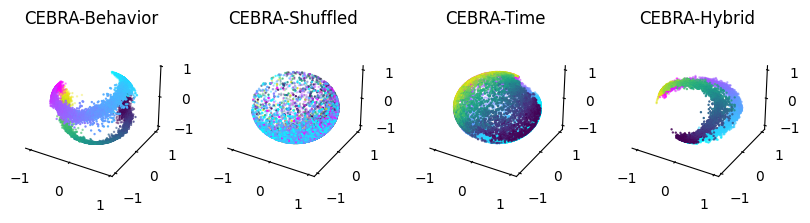
Visualize the embeddings from CEBRA-Behavior, CEBRA-Time and CEBRA-Hybrid#
[29]:
def plot_hippocampus(ax, embedding, label, gray = False, idx_order = (0,1,2)):
    r_ind = label[:,1] == 1
    l_ind = label[:,2] == 1

    if not gray:
        r_cmap = 'cool'
        l_cmap = 'viridis'
        r_c = label[r_ind, 0]
        l_c = label[l_ind, 0]
    else:
        r_cmap = None
        l_cmap = None
        r_c = 'gray'
        l_c = 'gray'

    idx1, idx2, idx3 = idx_order
    r=ax.scatter(embedding [r_ind,idx1],
               embedding [r_ind,idx2],
               embedding [r_ind,idx3],
               c=r_c,
               cmap=r_cmap, s=0.5)
    l=ax.scatter(embedding [l_ind,idx1],
               embedding [l_ind,idx2],
               embedding [l_ind,idx3],
               c=l_c,
               cmap=l_cmap, s=0.5)

    ax.grid(False)
    ax.xaxis.pane.fill = False
    ax.yaxis.pane.fill = False
    ax.zaxis.pane.fill = False
    ax.xaxis.pane.set_edgecolor('w')
    ax.yaxis.pane.set_edgecolor('w')
    ax.zaxis.pane.set_edgecolor('w')

    return ax
[30]:
%matplotlib inline
fig = plt.figure(figsize=(10,2))

ax1 = plt.subplot(141, projection='3d')
ax2 = plt.subplot(142, projection='3d')
ax3 = plt.subplot(143, projection='3d')
ax4 = plt.subplot(144, projection='3d')

ax1=plot_hippocampus(ax1, cebra_posdir3, hippocampus_pos.continuous_index)
ax2=plot_hippocampus(ax2, cebra_posdir_shuffled3, hippocampus_pos.continuous_index)
ax3=plot_hippocampus(ax3, cebra_time3, hippocampus_pos.continuous_index)
ax4=plot_hippocampus(ax4, cebra_hybrid, hippocampus_pos.continuous_index)

ax1.set_title('CEBRA-Behavior')
ax2.set_title('CEBRA-Shuffled')
ax3.set_title('CEBRA-Time')
ax4.set_title('CEBRA-Hybrid')
plt.show()
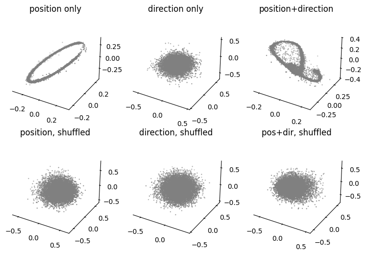
Hypothesis Testing: Train models with different hypothesis on position encoding of hippocampus.#
We will compare CEBRA-Behavior models trained with only position, only direction, both and the control models with shuffled behavior variables.
Here, we use the set model dimension; in the paper we used 3-64 on the hippocampus data (and found a consistent topology across these dimensions).
For the purpose of decoding later, we will use a splitted data (80% train, 20% test) and only use train set to train the models.
[31]:
output_dimension = 32 #setting this as a hyperparameter.
[32]:
def split_data(data, test_ratio):

    split_idx = int(len(data)* (1-test_ratio))
    neural_train = data.neural[:split_idx]
    neural_test = data.neural[split_idx:]
    label_train = data.continuous_index[:split_idx]
    label_test = data.continuous_index[split_idx:]

    return neural_train.numpy(), neural_test.numpy(), label_train.numpy(), label_test.numpy()

neural_train, neural_test, label_train, label_test = split_data(hippocampus_pos, 0.2)
[33]:
cebra_posdir_model = CEBRA(model_architecture='offset10-model',
                        batch_size=512,
                        learning_rate=3e-4,
                        temperature=1,
                        output_dimension=output_dimension,
                        max_iterations=max_iterations,
                        distance='cosine',
                        conditional='time_delta',
                        device='cuda_if_available',
                        verbose=True,
                        time_offsets=10)

cebra_pos_model = CEBRA(model_architecture='offset10-model',
                        batch_size=512,
                        learning_rate=3e-4,
                        temperature=1,
                        output_dimension=output_dimension,
                        max_iterations=max_iterations,
                        distance='cosine',
                        conditional='time_delta',
                        device='cuda_if_available',
                        verbose=True,
                        time_offsets=10)

cebra_dir_model = CEBRA(model_architecture='offset10-model',
                        batch_size=512,
                        learning_rate=3e-4,
                        temperature=1,
                        output_dimension=output_dimension,
                        max_iterations=max_iterations,
                        distance='cosine',
                        device='cuda_if_available',
                        verbose=True)
[34]:
# Train CEBRA-Behavior models with position, direction variable or both.
# We get train set embedding and test set embedding.

cebra_posdir_model.fit(neural_train, label_train)
cebra_posdir_train = cebra_posdir_model.transform(neural_train)
cebra_posdir_test = cebra_posdir_model.transform(neural_test)

cebra_pos_model.fit(neural_train, label_train[:,0])
cebra_pos_train = cebra_pos_model.transform(neural_train)
cebra_pos_test = cebra_pos_model.transform(neural_test)

cebra_dir_model.fit(neural_train, label_train[:,1])
cebra_dir_train = cebra_dir_model.transform(neural_train)
cebra_dir_test = cebra_dir_model.transform(neural_test)
pos: -0.8738 neg:  6.3912 total:  5.5174 temperature:  1.0000: 100%|██████████| 5000/5000 [00:53<00:00, 92.89it/s]
pos: -0.8701 neg:  6.4915 total:  5.6214 temperature:  1.0000: 100%|██████████| 5000/5000 [00:53<00:00, 94.05it/s]
pos: -0.8229 neg:  6.4787 total:  5.6559 temperature:  1.0000: 100%|██████████| 5000/5000 [00:53<00:00, 93.05it/s]
Train control models with shuffled behavior variables.#
[35]:
cebra_posdir_shuffled_model = CEBRA(model_architecture='offset10-model',
                        batch_size=512,
                        learning_rate=3e-4,
                        temperature=1,
                        output_dimension=output_dimension,
                        max_iterations=max_iterations,
                        distance='cosine',
                        conditional='time_delta',
                        device='cuda_if_available',
                        verbose=True,
                        time_offsets=10)

cebra_pos_shuffled_model = CEBRA(model_architecture='offset10-model',
                        batch_size=512,
                        learning_rate=3e-4,
                        temperature=1,
                        output_dimension=output_dimension,
                        max_iterations=max_iterations,
                        distance='cosine',
                        conditional='time_delta',
                        device='cuda_if_available',
                        verbose=True,
                        time_offsets=10)

cebra_dir_shuffled_model = CEBRA(model_architecture='offset10-model',
                        batch_size=512,
                        learning_rate=3e-4,
                        temperature=1,
                        output_dimension=output_dimension,
                        max_iterations=max_iterations,
                        distance='cosine',
                        device='cuda_if_available',
                        verbose=True)
[36]:
# Generate shuffled behavior labels for train set.
shuffled_posdir = np.random.permutation(label_train)
shuffled_pos = np.random.permutation(label_train[:,0])
shuffled_dir = np.random.permutation(label_train[:,1])

# Train the models with shuffled behavior variables and get train/test embeddings
cebra_posdir_shuffled_model.fit(neural_train, shuffled_posdir)
cebra_posdir_shuffled_train = cebra_posdir_shuffled_model.transform(neural_train)
cebra_posdir_shuffled_test = cebra_posdir_shuffled_model.transform(neural_test)

cebra_pos_shuffled_model.fit(neural_train, shuffled_pos)
cebra_pos_shuffled_train = cebra_pos_shuffled_model.transform(neural_train)
cebra_pos_shuffled_test = cebra_pos_shuffled_model.transform(neural_test)

cebra_dir_shuffled_model.fit(neural_train, shuffled_dir)
cebra_dir_shuffled_train = cebra_dir_shuffled_model.transform(neural_train)
cebra_dir_shuffled_test = cebra_dir_shuffled_model.transform(neural_test)
pos: -0.4657 neg:  6.5784 total:  6.1127 temperature:  1.0000: 100%|██████████| 5000/5000 [00:53<00:00, 93.57it/s]
pos: -0.4392 neg:  6.5624 total:  6.1232 temperature:  1.0000: 100%|██████████| 5000/5000 [00:52<00:00, 94.80it/s]
pos: -0.5164 neg:  6.5119 total:  5.9955 temperature:  1.0000: 100%|██████████| 5000/5000 [00:53<00:00, 93.56it/s]
Visualize embeddings from different hypothesis#
[37]:
cebra_pos_all = cebra_pos_model.transform(hippocampus_pos.neural)
cebra_dir_all = cebra_dir_model.transform(hippocampus_pos.neural)
cebra_posdir_all = cebra_posdir_model.transform(hippocampus_pos.neural)

cebra_pos_shuffled_all = cebra_pos_shuffled_model.transform(hippocampus_pos.neural)
cebra_dir_shuffled_all = cebra_dir_shuffled_model.transform(hippocampus_pos.neural)
cebra_posdir_shuffled_all = cebra_posdir_shuffled_model.transform(hippocampus_pos.neural)
[38]:
fig=plt.figure(figsize=(9,6))
ax1=plt.subplot(231, projection = '3d')
ax2=plt.subplot(232, projection = '3d')
ax3=plt.subplot(233, projection = '3d')
ax4=plt.subplot(234, projection = '3d')
ax5=plt.subplot(235, projection = '3d')
ax6=plt.subplot(236, projection = '3d')

ax1=plot_hippocampus(ax1, cebra_pos_all, hippocampus_pos.continuous_index, gray=True)
ax2=plot_hippocampus(ax2, cebra_dir_all, hippocampus_pos.continuous_index, gray=True)
ax3=plot_hippocampus(ax3, cebra_posdir_all,hippocampus_pos.continuous_index, gray=True)
ax4=plot_hippocampus(ax4, cebra_pos_shuffled_all, hippocampus_pos.continuous_index, gray=True)
ax5=plot_hippocampus(ax5, cebra_dir_shuffled_all, hippocampus_pos.continuous_index, gray=True)
ax6=plot_hippocampus(ax6, cebra_posdir_shuffled_all, hippocampus_pos.continuous_index, gray=True)

ax1.set_title('position only')
ax2.set_title('direction only')
ax3.set_title('position+direction')
ax4.set_title('position, shuffled')
ax5.set_title('direction, shuffled')
ax6.set_title('pos+dir, shuffled')

def ax_lim(ax):
    ax.set_xlim(-1,1)
    ax.set_ylim(-1,1)
    ax.set_zlim(-1,1)

plt.show()
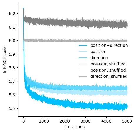
Visualize the loss of models trained with different hypothesis#
[39]:
fig = plt.figure(figsize=(5,5))
ax = plt.subplot(111)
ax.plot(cebra_posdir_model.state_dict_['loss'], c='deepskyblue', label = 'position+direction')
ax.plot(cebra_pos_model.state_dict_['loss'], c='deepskyblue', alpha = 0.3, label = 'position')
ax.plot(cebra_dir_model.state_dict_['loss'], c='deepskyblue', alpha=0.6,label = 'direction')
ax.plot(cebra_posdir_shuffled_model.state_dict_['loss'], c='gray', label = 'pos+dir, shuffled')
ax.plot(cebra_pos_shuffled_model.state_dict_['loss'], c='gray', alpha = 0.3, label = 'position, shuffled')
ax.plot(cebra_dir_shuffled_model.state_dict_['loss'],c='gray', alpha=0.6,label = 'direction, shuffled')

ax.spines['top'].set_visible(False)
ax.spines['right'].set_visible(False)
ax.set_xlabel('Iterations')
ax.set_ylabel('InfoNCE Loss')
plt.legend(bbox_to_anchor=(0.5,0.3), frameon = False )
plt.show()
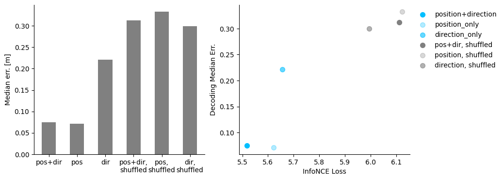
Decoding: we evaluate decoding performance of the different hypothesis models.#
[40]:
# Define decoding function with kNN decoder. For a simple demo, we will use the fixed number of neighbors 36.

from sklearn.neighbors import KNeighborsRegressor, KNeighborsClassifier
import sklearn.metrics

def decoding_pos_dir(emb_train, emb_test, label_train, label_test, n_neighbors=36):
    pos_decoder = KNeighborsRegressor(n_neighbors, metric = 'cosine')
    dir_decoder = KNeighborsClassifier(n_neighbors, metric = 'cosine')

    pos_decoder.fit(emb_train, label_train[:,0])
    dir_decoder.fit(emb_train, label_train[:,1])

    pos_pred = pos_decoder.predict(emb_test)
    dir_pred = dir_decoder.predict(emb_test)

    prediction =np.stack([pos_pred, dir_pred],axis = 1)

    test_score = sklearn.metrics.r2_score(label_test[:,:2], prediction)
    pos_test_err = np.median(abs(prediction[:,0] - label_test[:, 0]))
    pos_test_score = sklearn.metrics.r2_score(label_test[:, 0], prediction[:,0])

    return test_score, pos_test_err, pos_test_score
Decode the position and direction from the trained hypothesis models
[41]:
cebra_posdir_decode = decoding_pos_dir(cebra_posdir_train, cebra_posdir_test, label_train, label_test)
cebra_pos_decode = decoding_pos_dir(cebra_pos_train, cebra_pos_test, label_train, label_test)
cebra_dir_decode = decoding_pos_dir(cebra_dir_train, cebra_dir_test, label_train, label_test)
cebra_posdir_shuffled_decode = decoding_pos_dir(cebra_posdir_shuffled_train, cebra_posdir_shuffled_test, label_train, label_test)
cebra_pos_shuffled_decode = decoding_pos_dir(cebra_pos_shuffled_train, cebra_pos_shuffled_test, label_train, label_test)
cebra_dir_shuffled_decode = decoding_pos_dir(cebra_dir_shuffled_train, cebra_dir_shuffled_test, label_train, label_test)
Visualize the decoding results and loss - decoding performance#
[42]:
fig = plt.figure(figsize=(10,4))
ax1= plt.subplot(121)
ax1.bar(np.arange(6),
        [cebra_posdir_decode[1], cebra_pos_decode[1], cebra_dir_decode[1],
         cebra_posdir_shuffled_decode[1], cebra_pos_shuffled_decode[1], cebra_dir_shuffled_decode[1]],
         width = 0.5, color = 'gray')
ax1.spines['top'].set_visible(False)
ax1.spines['right'].set_visible(False)
ax1.set_xticks(np.arange(6))
ax1.set_xticklabels(['pos+dir', 'pos', 'dir', 'pos+dir,\nshuffled', 'pos,\nshuffled', 'dir,\nshuffled'])
ax1.set_ylabel('Median err. [m]')

ax2 = plt.subplot(122)
ax2.scatter(cebra_posdir_model.state_dict_['loss'][-1],cebra_posdir_decode[1], s=50, c='deepskyblue', label = 'position+direction')
ax2.scatter(cebra_pos_model.state_dict_['loss'][-1],cebra_pos_decode[1], s=50, c='deepskyblue', alpha = 0.3, label = 'position_only')
ax2.scatter(cebra_dir_model.state_dict_['loss'][-1],cebra_dir_decode[1], s=50, c='deepskyblue', alpha=0.6,label = 'direction_only')
ax2.scatter(cebra_posdir_shuffled_model.state_dict_['loss'][-1],cebra_posdir_shuffled_decode[1], s=50, c='gray', label = 'pos+dir, shuffled')
ax2.scatter(cebra_pos_shuffled_model.state_dict_['loss'][-1],cebra_pos_shuffled_decode[1], s=50, c='gray', alpha = 0.3, label = 'position, shuffled')
ax2.scatter(cebra_dir_shuffled_model.state_dict_['loss'][-1],cebra_dir_shuffled_decode[1], s=50, c='gray', alpha=0.6,label = 'direction, shuffled')

ax2.spines['top'].set_visible(False)
ax2.spines['right'].set_visible(False)
ax2.set_xlabel('InfoNCE Loss')
ax2.set_ylabel('Decoding Median Err.')
plt.legend(bbox_to_anchor=(1,1), frameon = False )
plt.show()
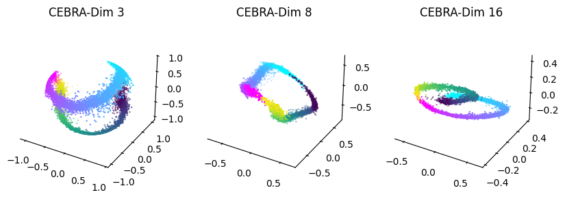
Persistent cohomology analysis with CEBRA embeddings of varying output dimensions:#
Train additional CEBRA-Behavior with dimensions 8, 16#
[43]:
cebra_posdir8_model= CEBRA(model_architecture='offset10-model',
                        batch_size=512,
                        learning_rate=3e-4,
                        temperature=1,
                        output_dimension=8,
                        max_iterations=max_iterations,
                        distance='cosine',
                        conditional='time_delta',
                        device='cuda_if_available',
                        verbose=True,
                        time_offsets=10)
cebra_posdir16_model = CEBRA(model_architecture='offset10-model',
                        batch_size=512,
                        learning_rate=3e-4,
                        temperature=1,
                        output_dimension=16,
                        max_iterations=max_iterations,
                        distance='cosine',
                        conditional='time_delta',
                        device='cuda_if_available',
                        verbose=True,
                        time_offsets=10)
[44]:
cebra_posdir8_model.fit(hippocampus_pos.neural, hippocampus_pos.continuous_index.numpy())
cebra_posdir8 = cebra_posdir8_model.transform(hippocampus_pos.neural)

cebra_posdir16_model.fit(hippocampus_pos.neural, hippocampus_pos.continuous_index.numpy())
cebra_posdir16 = cebra_posdir16_model.transform(hippocampus_pos.neural)
pos: -0.8834 neg:  6.4076 total:  5.5242 temperature:  1.0000: 100%|██████████| 5000/5000 [00:52<00:00, 94.70it/s]
pos: -0.9017 neg:  6.3850 total:  5.4834 temperature:  1.0000: 100%|██████████| 5000/5000 [00:52<00:00, 95.00it/s]
Plotting the results:#
[45]:
fig = plt.figure(figsize = (10,3), dpi = 100)

ax1 = plt.subplot(131,projection='3d')
ax2 = plt.subplot(132, projection = '3d')
ax3 = plt.subplot(133, projection = '3d')

ax1=plot_hippocampus(ax1, cebra_posdir3, hippocampus_pos.continuous_index)
ax2=plot_hippocampus(ax2, cebra_posdir8, hippocampus_pos.continuous_index)
ax3=plot_hippocampus(ax3, cebra_posdir16, hippocampus_pos.continuous_index)

ax1.set_title('CEBRA-Dim 3')
ax2.set_title('CEBRA-Dim 8')
ax3.set_title('CEBRA-Dim 16')
plt.show()
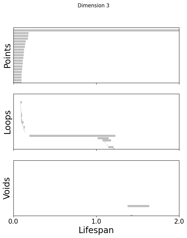
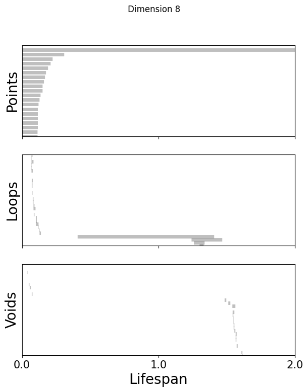
Topological Data Analysis:#
Get random 1000 points of embeddings and do persistent cohomology analysis upto H1#
note this requires the ripser package.
If you previously installed DREiMac (such as running this notebook before, there are some dependency clashes with ripser, so you need to uninstall it first, and reinstall risper:
[46]:
#!pip uninstall -y dreimac
#!pip uninstall -y cebra
#!pip uninstall -y ripser
[47]:
#!pip install ripser

#Depending on your system, this can cause errors.
#Thus if issues please follow these instructions directly: https://pypi.org/project/ripser/
import ripser
if you get the error
ValueError: numpy.ndarray size changed, may indicate binary incompatibility. Expected 96 from C header, got 80 from PyObject, please delete the folders from DREiMac and run the cell above again.
[48]:
maxdim=1 ## Set to 2 to compute upto H2. The computing time is considerably longer. For quick demo upto H1, set it to 1.
np.random.seed(111)
random_idx=np.random.permutation(np.arange(len(cebra_posdir3)))[:1000]
topology_dimension = {}
for embedding in [cebra_posdir3, cebra_posdir8, cebra_posdir16]:
    ripser_output=ripser.ripser(embedding[random_idx], maxdim=maxdim, coeff=47)
    dimension = embedding.shape[1]
    topology_dimension[dimension] = ripser_output
If you want to visualize the pre-computed persistent co-homology result:#
preloading saves quite a bit of time; to adapt to your own datasets please set topology_dimension and random_inx.
[49]:
CURRENT_DIR = '/content/'
import os

preload=pd.read_hdf(os.path.join(CURRENT_DIR,'rat_demo_example_output.h5'))
topology_dimension = preload['topology']
topology_random_dimension = preload['topology_random']
random_idx = preload['embedding']['random_idx']
maxdim=2
[50]:
def plot_barcode(topology_result, maxdim):
    fig, axs = plt.subplots(maxdim+1, 1, sharex=True, figsize=(7, 8))
    axs[0].set_xlim(0,2)
    cocycle = ["Points", "Loops", "Voids"]
    for k in range(maxdim+1):
        bars = topology_result['dgms'][k]
        bars[bars == np.inf] = 10
        lc = (
            np.vstack(
                [
                    bars[:, 0],
                    np.arange(len(bars), dtype=int) * 6,
                    bars[:, 1],
                    np.arange(len(bars), dtype=int) * 6,
                ]
            )
            .swapaxes(1, 0)
            .reshape(-1, 2, 2)
        )
        line_segments = LineCollection(lc, linewidth=5, color="gray", alpha=0.5)
        axs[k].set_ylabel(cocycle[k], fontsize=20)
        if k == 0:
            axs[k].set_ylim(len(bars) * 6 - 120, len(bars) * 6)
        elif k == 1:
            axs[k].set_ylim(0, len(bars) * 1 - 30)
        elif k == 2:
            axs[k].set_ylim(0, len(bars) * 6 + 10)
        axs[k].add_collection(line_segments)
        axs[k].set_yticks([])
        if k == 2:
            axs[k].set_xticks(np.linspace(0, 2, 3), np
                              .linspace(0, 2, 3), fontsize=15)
            axs[k].set_xlabel("Lifespan", fontsize=20)

    return fig
[51]:
%matplotlib inline
for k in [3,8,16]:
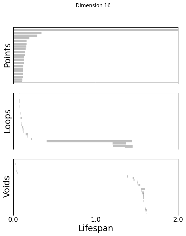
fig=plot_barcode(topology_dimension[k], maxdim)
fig.suptitle(f'Dimension {k}')
[52]:
from persim import plot_diagrams

def read_lifespan(ripser_output, dim):
    dim_diff = ripser_output['dgms'][dim][:, 1] - ripser_output['dgms'][dim][:, 0]
    if dim == 0:
        return dim_diff[~np.isinf(dim_diff)]
    else:
        return dim_diff

def get_max_lifespan(ripser_output_list, maxdim):
    lifespan_dic = {i: [] for i in range(maxdim+1)}
    for f in ripser_output_list:
        for dim in range(maxdim+1):
            lifespan = read_lifespan(f, dim)
            lifespan_dic[dim].extend(lifespan)
    return [max(lifespan_dic[i]) for i in range(maxdim+1)], lifespan_dic

def get_betti_number(ripser_output, shuffled_max_lifespan):
    bettis=[]
    for dim in range(len(ripser_output['dgms'])):
        lifespans=ripser_output['dgms'][dim][:, 1] - ripser_output['dgms'][dim][:, 0]
        betti_d = sum(lifespans > shuffled_max_lifespan[dim] * 1.1)
        bettis.append(betti_d)
    return bettis
def plot_lifespan(topology_dgms, shuffled_max_lifespan, ax, label_vis, maxdim):
    plot_diagrams(
        topology_dgms,
        ax=ax,
        legend=True,
    )

    ax.plot(
        [
            -0.5,
            2,
        ],
        [-0.5 + shuffled_max_lifespan[0], 2 + shuffled_max_lifespan[0]],
        color="C0",
        linewidth=3,
        alpha=0.5,

    )
    ax.plot(
        [
            -0.5,
            2,
        ],
        [-0.5 + shuffled_max_lifespan[1], 2 + shuffled_max_lifespan[1]],
        color="orange",
        linewidth=3,
        alpha=0.5,

    )
    if maxdim == 2:
        ax.plot(
            [-0.50, 2],
            [-0.5 + shuffled_max_lifespan[2], 2 + shuffled_max_lifespan[2]],
            color="green",
            linewidth=3,
            alpha=0.5,
        )
    ax.set_xlabel("Birth", fontsize=15)
    ax.set_xticks([0, 1, 2])
    ax.set_xticklabels([0, 1, 2])
    ax.tick_params(labelsize=13)
    if label_vis:
        ax.set_ylabel("Death", fontsize=15)
    else:
        ax.set_ylabel("")
[53]:
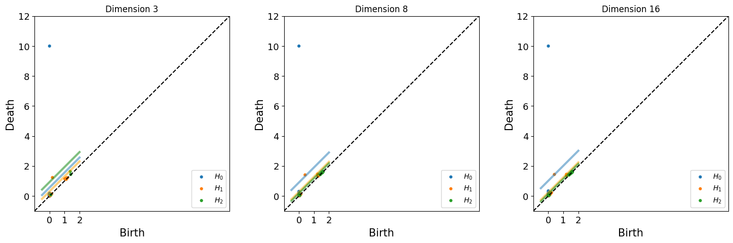
fig = plt.figure(figsize=(18,5))
for n, dim in enumerate([3,8,16]):
    shuffled_max_lifespan, lifespan_dic = get_max_lifespan(topology_random_dimension[dim], maxdim)
    ax = fig.add_subplot(1,3,n+1)
    ax.set_title(f'Dimension {dim}')
    plot_lifespan(topology_dimension[dim]['dgms'], shuffled_max_lifespan, ax, True, maxdim)
    print(f"Betti No. for dimension {dim}: {get_betti_number(topology_dimension[dim], shuffled_max_lifespan)}")
Betti No. for dimension 3: [1, 1, 0]
Betti No. for dimension 8: [1, 1, 0]
Betti No. for dimension 16: [1, 1, 0]
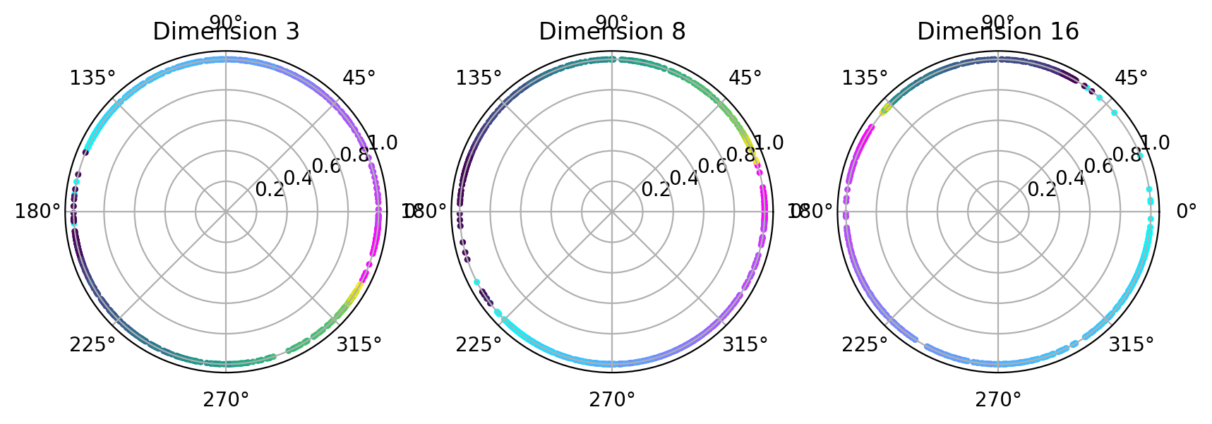
Visualize topology-preserving circular coordinates from the first co-cycle.#
This requires the DREiMac codebase. Here, we show you how to install their package:
[54]:
from dreimac import CircularCoords
[55]:
%matplotlib inline

prime = 47
dimension = [3,8,16]
fig, axs = plt.subplots(1, 3, figsize=(10,3), dpi=200, subplot_kw={'projection': 'polar'})
label = hippocampus_pos.continuous_index[random_idx]
r_ind = label[:,1]==1
l_ind = label[:,2]==1
for i, embedding in enumerate([cebra_posdir3, cebra_posdir8, cebra_posdir16]):
    rat_emb=embedding[random_idx]
    cc = CircularCoords(rat_emb, 1000, prime = prime, )
    radial_angle=cc.get_coordinates(cocycle_idx=[0])
    r = np.ones(1000)
    right=axs[i].scatter(radial_angle[r_ind], r[r_ind], s=5, c = label[r_ind,0], cmap = 'cool')
    left=axs[i].scatter(radial_angle[l_ind], r[l_ind], s=5, c = label[l_ind,0], cmap = 'viridis')
    axs[i].set_title(f'Dimension {dimension[i]}')
plt.show()
Visualize Polar coordinate (radial angle) vs. Position#
if you want to preload our data, run the following, otherwise skip this cell:
[56]:
cebra_pos3 = preload['embedding'][3]
cebra_pos8 = preload['embedding'][8]
cebra_pos16 = preload['embedding'][16]
[57]:
radial_angles = {}
for i, embedding in enumerate([cebra_pos3, cebra_pos8, cebra_pos16]):
    rat_emb=embedding[random_idx]
    cc = CircularCoords(rat_emb, 1000, prime = prime, )
    out=cc.get_coordinates()
    radial_angles[dimension[i]] = out
[58]:
%matplotlib inline
for k in radial_angles.keys():
    fig=plt.figure(figsize=(7,6))
    plt.subplots_adjust(wspace=0.3)
    fig.suptitle(f'Dimension {k}')
    ax1=plt.subplot(121)
    ax1.scatter(radial_angles[k][r_ind], label[r_ind,0], s=1, c = 'gray')
    ax1.set_xlabel('Radial angle [rad]')
    ax1.set_ylabel('Position [m]')
    ax2=plt.subplot(122)
    ax2.scatter(radial_angles[k][l_ind], label[l_ind,0], s=1, c= 'gray')
    ax2.set_xlabel('Radial angle [rad]')
    ax2.set_ylabel('Position [m]')
plt.show()
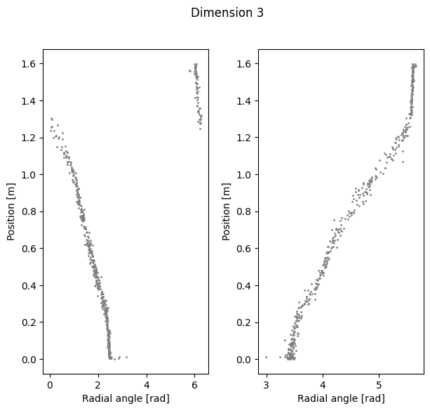
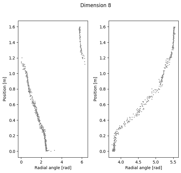
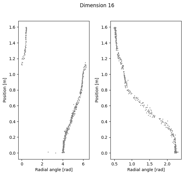
Compute linear correlation between computed coordinate and the position#
[59]:
import sklearn.linear_model
def lin_regression(radial_angles, labels):
    def _to_cartesian(radial_angles):
        x = np.cos(radial_angles)
        y = np.sin(radial_angles)
        return np.vstack([x,y]).T
    cartesian = _to_cartesian(radial_angles)
    lin = sklearn.linear_model.LinearRegression()
    lin.fit(cartesian, labels)

    return lin.score(cartesian, labels)
[60]:
for k in radial_angles.keys():
    print(f'Dimension {k} Cycle angle into position')
    print(f'Right R2: {lin_regression(radial_angles[k][r_ind], label[r_ind,0])}')
    print(f'Left R2: {lin_regression(radial_angles[k][l_ind], label[l_ind,0])}')
    print(f'Total R2: {lin_regression(radial_angles[k], label[:,0])}')
Dimension 3 Cycle angle into position
Right R2: 0.9739516384371666
Left R2: 0.9703212139226258
Total R2: 0.9706971877624279
Dimension 8 Cycle angle into position
Right R2: 0.964004591807784
Left R2: 0.9637490253487142
Total R2: 0.9110782393146737
Dimension 16 Cycle angle into position
Right R2: 0.9569758425034549
Left R2: 0.9507297439954339
Total R2: 0.8680615520754118
Interactive plot to explore co-cycles and circular coordinates.#
Top left panel is a lifespan diagram of persistent co-homology analysis.
Bottom left panel is a visualization of the first 2 dimensions of the used 1000 embedding points.
Bottom right panel is a circular coordinate obtained from the co-cycles.
For more information: ctralie/DREiMac
[61]:
## change the embedding to use. Here, we look at 3D embedding for posdir3 (position+dir, dim 3):
X=cebra_posdir3[random_idx]

%matplotlib notebook
rl_stack=np.vstack([X[r_ind], X[l_ind]])
label_stack = np.vstack([label[r_ind], label[l_ind]])

c1 = plt.get_cmap('cool')
C1 = c1(label[r_ind,0])
c2 = plt.get_cmap('viridis')
C2 = c2(label[l_ind,0])

C = np.vstack([C1,C2])

def plot_circles(ax):
    ax.scatter(rl_stack[:, 0], rl_stack[:, 1], c=C)


cc = CircularCoords(rl_stack, 1000, prime = prime)
cc.plot_torii(C, coords_info=2, plots_in_one=3, lowerleft_plot=plot_circles)
/usr/local/lib/python3.11/dist-packages/dreimac/emcoords.py:66: UserWarning:

Could not accurately determine screen size