You can download and run the notebook locally:
Extended Data Figure 1: Overview of datasets, synthetic data, & original pi-VAE implementation vs. modified conv-pi-VAE#
import plot and data loading dependencies#
[1]:
import sys
import numpy as np
import matplotlib.pyplot as plt
import pandas as pd
from matplotlib.lines import Line2D
from matplotlib.patches import Circle
import seaborn as sns
import sklearn.linear_model
[2]:
data = pd.read_hdf("../data/EDFigure1.h5")
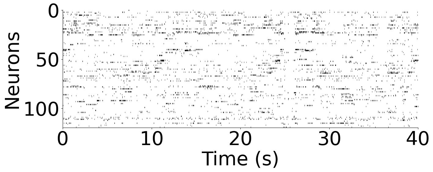
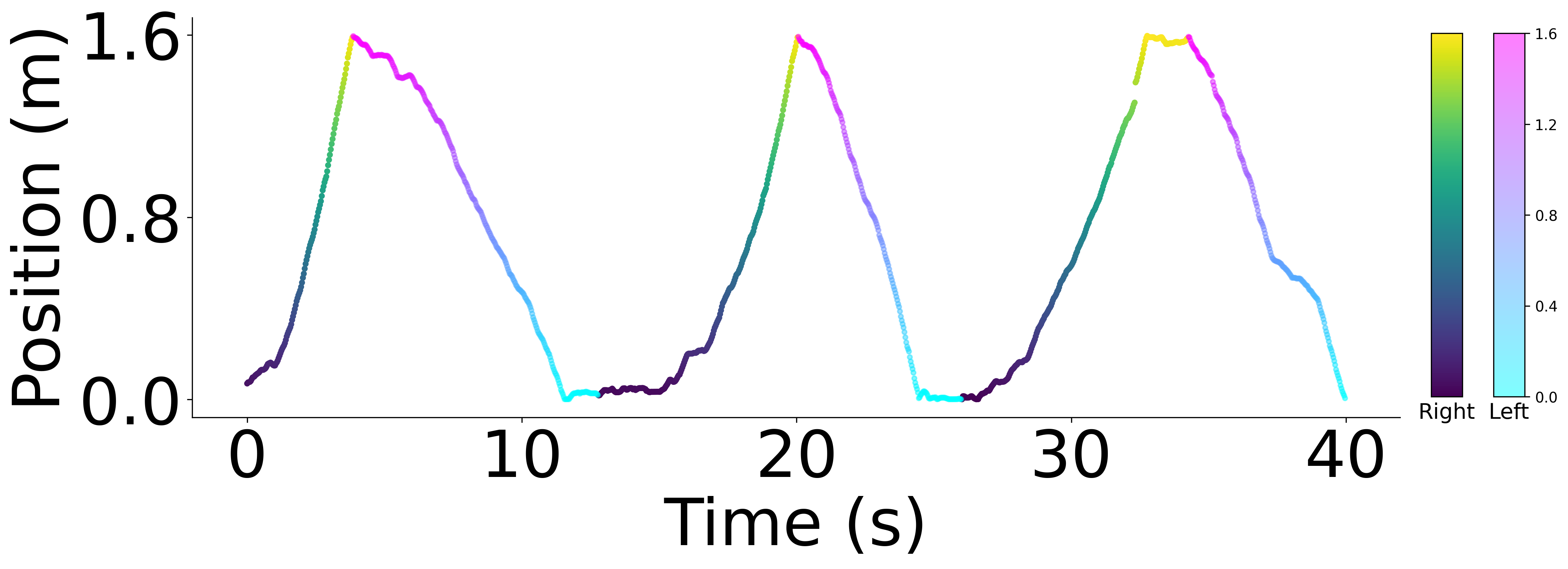
Plot example data the rat hippocampus dataset, from rat 1: neurons and behavior#
[3]:
rat_neural = data["rat"]["neural"]
rat_behavior = data["rat"]["behavior"]
fig = plt.figure(figsize=(15, 5))

ax = plt.subplot(111)
ax.imshow(rat_neural.T, aspect="auto", cmap="gray_r", vmax=1)
plt.ylabel("Neurons", fontsize=45)
plt.xlabel("Time (s)", fontsize=45)
plt.xticks(np.linspace(0, len(rat_neural), 5), np.arange(0, 45, 10))
plt.yticks([0, 50, 100], [0, 50, 100])
plt.xticks(fontsize=45)
plt.yticks(fontsize=45)

ax.spines["right"].set_visible(False)
ax.spines["top"].set_visible(False)

r = rat_behavior[:, 1] == 1
l = rat_behavior[:, 1] == 0
fig = plt.figure(figsize=(15, 5), dpi=300)
ax = plt.subplot(111)
ax_r = ax.scatter(
    np.arange(len(rat_behavior))[r] * 0.025,
    rat_behavior[r, 0],
    c=rat_behavior[r, 0],
    cmap="viridis",
    s=10,
)
ax_l = ax.scatter(
    np.arange(len(rat_behavior))[l] * 0.025,
    rat_behavior[l, 0],
    c=rat_behavior[l, 0],
    cmap="cool",
    s=10,
    alpha=0.5,
)

ax.spines["right"].set_visible(False)
ax.spines["top"].set_visible(False)

plt.ylabel("Position (m)", fontsize=45)
plt.xlabel("Time (s)", fontsize=45)
plt.xticks(fontsize=45)
plt.yticks(np.linspace(0, 1.6, 3), fontsize=45)
plt.xticks(np.linspace(0, len(rat_behavior), 5) * 0.025, np.arange(0, 45, 10))
cb_r_axes = fig.add_axes([0.92, 0.15, 0.02, 0.7])
cb_l_axes = fig.add_axes([0.96, 0.15, 0.02, 0.7])
cb_r = plt.colorbar(ax_r, cax=cb_r_axes, boundaries=np.linspace(0, 1.6, 200))
cb_l = plt.colorbar(
    ax_l,
    cax=cb_l_axes,
    boundaries=np.linspace(0, 1.6, 200),
    ticks=np.linspace(0, 1.6, 5),
)
cb_r.set_ticks([])

cb_r.ax.set_xlabel("Right", fontsize=15)
cb_l.ax.set_xlabel("Left", fontsize=15)
[3]:
Text(0.5, 0, 'Left')
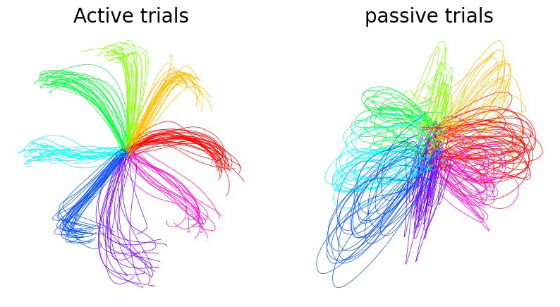
Plot example behavior data from the monkey S1 dataset#
[4]:
active_target = data["monkey"]["behavior"]["active"]["target"]
passive_target = data["monkey"]["behavior"]["passive"]["target"]
active_pos = data["monkey"]["behavior"]["active"]["position"]
passive_pos = data["monkey"]["behavior"]["passive"]["position"]

fig = plt.figure(figsize=(10, 5))

ax1 = plt.subplot(1, 2, 1)
ax1.set_title("Active trials", fontsize=20)
for n, i in enumerate(active_pos.reshape(-1, 600, 2)):
    k = active_target[n * 600]
    ax1.plot(i[:, 0], i[:, 1], color=plt.cm.hsv(1 / 8 * k), linewidth=0.5)
    ax1.spines["right"].set_visible(False)
    ax1.spines["top"].set_visible(False)
plt.axis("off")
ax2 = plt.subplot(1, 2, 2)
ax2.set_title("passive trials", fontsize=20)
for n, i in enumerate(passive_pos.reshape(-1, 600, 2)):
    k = passive_target[n * 600]
    ax2.plot(i[:, 0], i[:, 1], color=plt.cm.hsv(1 / 8 * k), linewidth=0.5)
plt.axis("off")
[4]:
(-7.249750447273255, 6.267432045936585, -4.10022519826889, 3.132592189311981)
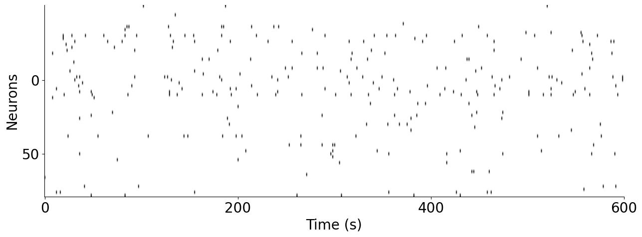
Plot example neural data from the monkey S1 dataset#
[5]:
fig = plt.figure(figsize=(15, 5))
ephys = data["monkey"]["neural"]
ax = plt.subplot(111)
ax.imshow(ephys[:600].T, aspect="auto", cmap="gray_r", vmax=1, vmin=0)
plt.ylabel("Neurons", fontsize=20)
plt.xlabel("Time (s)", fontsize=20)
plt.xticks([0, 200, 400, 600], ["0", "200", "400", "600"], fontsize=20)
plt.yticks(fontsize=20)
plt.yticks([25, 50], ["0", "50"])

ax.spines["right"].set_visible(False)
ax.spines["top"].set_visible(False)
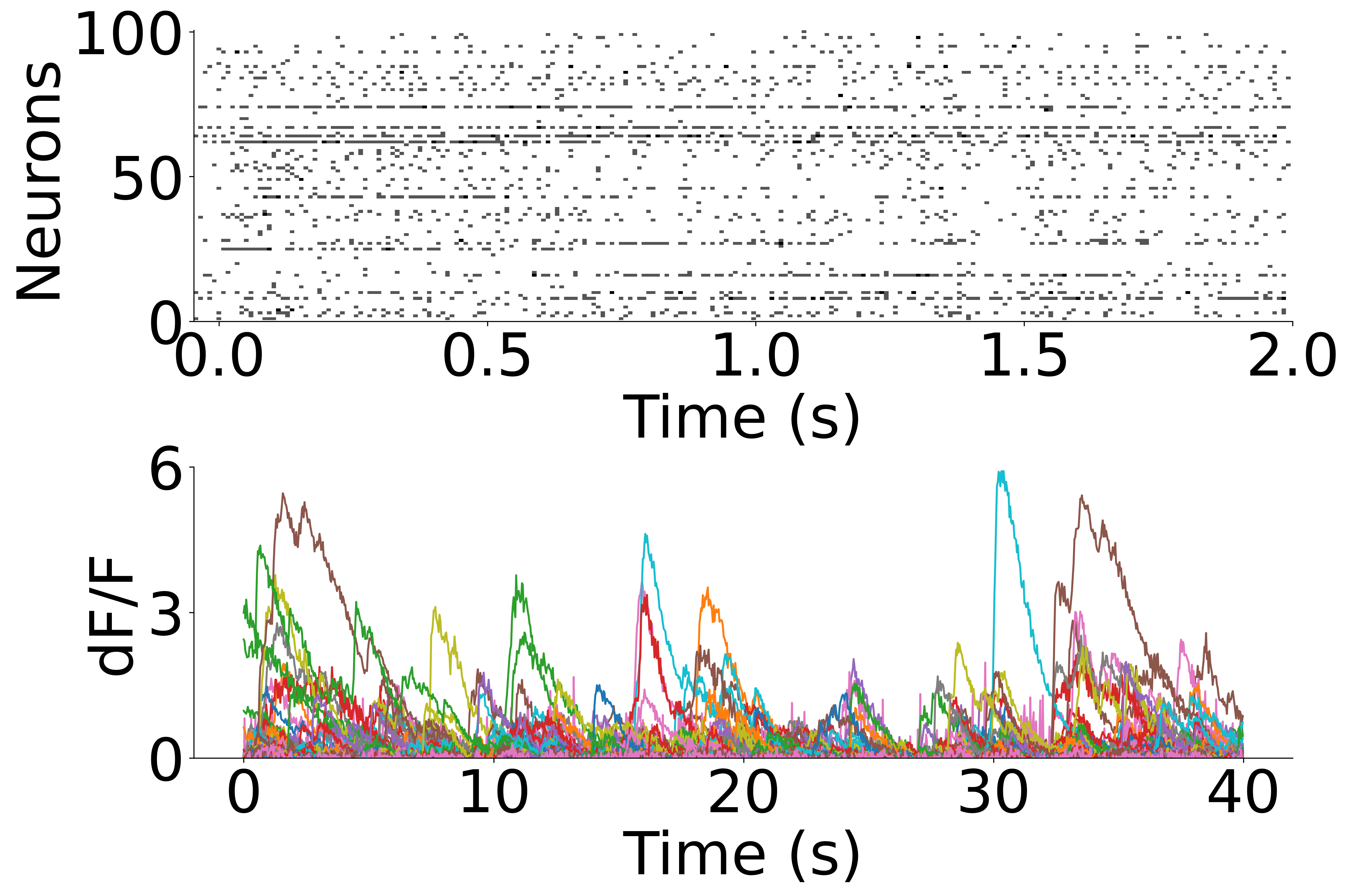
Plot example behavior data from the Allen datasets: Neuropixels & 2P calcium imaging#
[6]:
neuropixel = data["mouse"]["neural"]["np"]
ca = data["mouse"]["neural"]["ca"]
fig = plt.figure(figsize=(15, 10), dpi=300)
plt.subplots_adjust(hspace=0.5)
ax1 = plt.subplot(2, 1, 1)
plt.imshow(neuropixel[:100, :240], aspect="auto", vmin=0, vmax=1.5, cmap="gray_r")
plt.ylabel("Neurons", fontsize=45)
plt.xlabel("Time (s)", fontsize=45)
plt.xticks(np.linspace(5, 240, 5), np.linspace(0, 2, 5))
plt.yticks([0, 50, 100], [100, 50, 0])
plt.xticks(fontsize=45)
plt.yticks(fontsize=45)
ax1.spines["right"].set_visible(False)
ax1.spines["top"].set_visible(False)

ax2 = plt.subplot(2, 1, 2)
ax2.plot(ca.T)
plt.ylabel("dF/F", fontsize=45)
plt.xlabel("Time (s)", fontsize=45)
plt.ylim(0, 6)
# plt.xlim(0,1200)
plt.xticks(
    np.linspace(0, 1200, 5),
    np.linspace(0, 40, 5).astype(int),
    fontsize=20,
)
plt.yticks([0, 3, 6], [0, 3, 6], fontsize=45)
plt.xticks(fontsize=45)
ax2.spines["right"].set_visible(False)
ax2.spines["top"].set_visible(False)
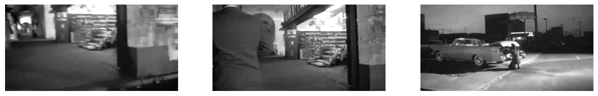
Plot example video (natural movie 1) data from the Allen datasets#
[7]:
plt.figure(figsize=(15, 5))
for n, i in enumerate(data["mouse"]["behavior"]):
    ax = plt.subplot(1, 3, n + 1)
    ax.imshow(i, cmap="gray")
    plt.axis("off")
Synthetic data experiments: benchmarking#
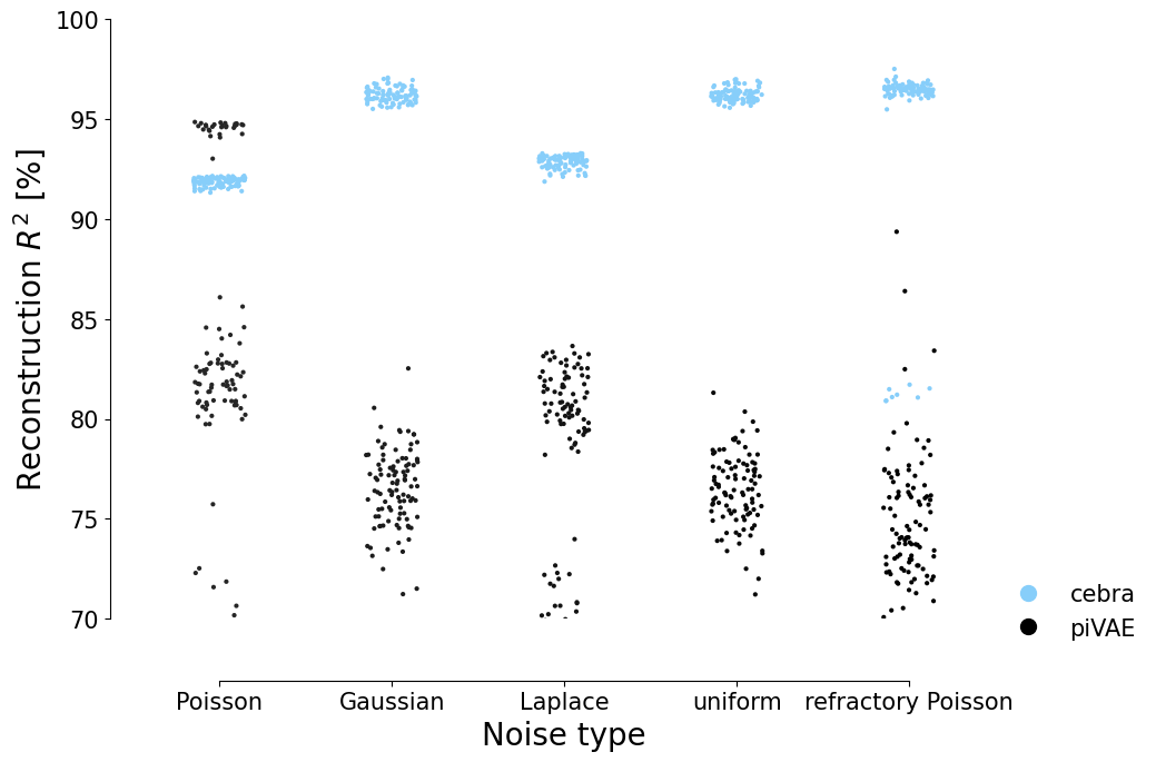
we test 5 different types of synthetic data:
[8]:
def reindex(
    dic, list_name=["poisson", "gaussian", "laplace", "uniform", "refractory_poisson"]
):
    return rename(pd.DataFrame(dic).T.reindex(list_name).T * 100)


def rename(df):
    return df.rename(
        columns={
            "poisson": "Poisson",
            "gaussian": "Gaussian",
            "laplace": "Laplace",
            "uniform": "uniform",
            "refractory_poisson": "refractory Poisson",
        }
    )
Plot the 100 runs (seeds) for both piVAE and CEBRA on the 5 datasets:#
[9]:
data_pivae = data["noise_exp"]["pivae"]
data_cebra = data["noise_exp"]["cebra"]
fig = plt.figure(figsize=(10, 7))

ax = plt.subplot(111)

sns.stripplot(
    data=reindex(data_pivae["x-s"]["poisson"]),
    jitter=0.15,
    s=3,
    color="black",
    label="pi_vae",
)
sns.stripplot(
    data=reindex(data_cebra["x-s"]["infonce"]),
    jitter=0.15,
    s=3,
    palette=["lightskyblue"],
    label="cebra",
    hue = None
)


ax.set_ylabel("Reconstruction $R^2$ [%]", fontsize=20)
ax.set_xlabel("Noise type", fontsize=20)
ax.spines["right"].set_visible(False)
ax.spines["top"].set_visible(False)
ax.set_ylim((70, 100))
ax.tick_params(axis="both", which="major", labelsize=15)
legend_elements = [
    Line2D(
        [0],
        [0],
        markersize=10,
        linestyle="none",
        marker="o",
        color="lightskyblue",
        label="cebra",
    ),
    Line2D(
        [0],
        [0],
        markersize=10,
        linestyle="none",
        marker="o",
        color="black",
        label="piVAE",
    ),
]
ax.legend(handles=legend_elements, loc=(1.0, -0.05), frameon=False, fontsize=15)
sns.despine(
    left=False,
    right=True,
    bottom=False,
    top=True,
    trim=True,
    offset={"bottom": 40, "left": 15},
)
plt.savefig("distribution_reconstruction.png", transparent=True, bbox_inches="tight")
/Users/celiabenquet/miniconda/envs/repro/lib/python3.10/site-packages/seaborn/categorical.py:166: FutureWarning: Setting a gradient palette using color= is deprecated and will be removed in version 0.13. Set `palette='dark:black'` for same effect.
  warnings.warn(msg, FutureWarning)
/var/folders/d7/97cvt_0n63j6tygn4f5mfkzw0000gn/T/ipykernel_74998/4160691022.py:14: UserWarning:
The palette list has fewer values (1) than needed (5) and will cycle, which may produce an uninterpretable plot.
  sns.stripplot(
Compute statistics
[10]:
from statsmodels.stats.oneway import anova_oneway
import statsmodels.api as sm
from statsmodels.formula.api import ols

keys = data_pivae["x-s"]["poisson"].keys()
assert data_cebra["x-s"]["infonce"].keys() == keys

pivae_frame = reindex(data_pivae["x-s"]["poisson"]).unstack().to_frame().reset_index()
cebra_frame = reindex(data_cebra["x-s"]["infonce"]).unstack().to_frame().reset_index()
pivae_frame.columns = 'dataset', 'drop', 'r2'
pivae_frame['model'] = 'pivae'
cebra_frame.columns = 'dataset', 'drop', 'r2'
cebra_frame['model'] = 'cebra'

all_data = pd.concat([pivae_frame, cebra_frame], axis = 0)\
  .drop(columns = ['drop',])
[11]:
import scipy.stats
import statsmodels.stats.oneway
import statsmodels.stats.multitest
import functools

grouped_data = all_data.pivot_table(
  "r2",
  index = 'dataset',
  columns = 'model',
  aggfunc = list
)

# comparison by t-test for each of the experiments
results = []
for index in grouped_data.index:
  test_data = [
    grouped_data.loc[index, 'pivae'],
    grouped_data.loc[index, 'cebra']
  ]

  # Test for equal variance
  # https://en.wikipedia.org/wiki/Brown%E2%80%93Forsythe_test
  result = statsmodels.stats.oneway.test_scale_oneway(
    test_data, method='bf', center='median',
    transform='abs', trim_frac_mean=0.0,
    trim_frac_anova=0.0
  )

  # Test if sign. improvement
  stats = scipy.stats.ttest_ind(
    *test_data,
    equal_var = False
  )

  results.append(dict(
    dataset = index,
    variance_df = result.df,
    variance_F = result.statistic,
    variance_p1 = result.pvalue,
    variance_p2 = result.pvalue2,
    #mean_report = f'F({},{}) = {}, p = {}'
    mean_t = stats.statistic,
    mean_p = stats.pvalue,
  )
  )


results = pd.DataFrame(results)

print("Uncorrected stats")
with pd.option_context('display.max_rows', None, 'display.max_columns', None, 'display.max_colwidth', None):
    display(results)

correct_pvalues = functools.partial(
  statsmodels.stats.multitest.multipletests,
  alpha=0.05, method='holm', is_sorted=False, returnsorted=False
)

reject, results['mean_p'], _, _ = correct_pvalues(results['mean_p'].values)
assert all(reject)
reject, results['variance_p1'], _, _ = correct_pvalues(results['variance_p1'].values)
assert all(reject)
reject, results['variance_p2'], _, _ = correct_pvalues(results['variance_p2'].values)
assert all(reject)

print("Corrected stats (Bonferroni-Holm)")
display(results)
Uncorrected stats
| dataset | variance_df | variance_F | variance_p1 | variance_p2 | mean_t | mean_p | |
|---|---|---|---|---|---|---|---|
| 0 | Gaussian | (1.0, 105.43278258979824) | 105.601855 | 1.406860e-17 | 1.406860e-17 | -101.373592 | 3.724708e-107 |
| 1 | Laplace | (1.0000000000000002, 99.63294297266972) | 61.353754 | 5.288466e-12 | 5.288466e-12 | -30.554650 | 1.656493e-52 |
| 2 | Poisson | (0.9999999999999999, 99.11379313255243) | 83.872178 | 7.430972e-15 | 7.430972e-15 | -10.534166 | 7.351225e-18 |
| 3 | refractory Poisson | (1.0000000000000002, 156.2456086071841) | 4.022731 | 4.661709e-02 | 4.661709e-02 | -38.657842 | 7.248700e-91 |
| 4 | uniform | (1.0000000000000002, 105.587408572814) | 110.764156 | 3.827807e-18 | 3.827807e-18 | -107.465767 | 2.475565e-109 |
Corrected stats (Bonferroni-Holm)
| dataset | variance_df | variance_F | variance_p1 | variance_p2 | mean_t | mean_p | |
|---|---|---|---|---|---|---|---|
| 0 | Gaussian | (1.0, 105.43278258979824) | 105.601855 | 5.627440e-17 | 5.627440e-17 | -101.373592 | 1.489883e-106 |
| 1 | Laplace | (1.0000000000000002, 99.63294297266972) | 61.353754 | 1.057693e-11 | 1.057693e-11 | -30.554650 | 3.312985e-52 |
| 2 | Poisson | (0.9999999999999999, 99.11379313255243) | 83.872178 | 2.229292e-14 | 2.229292e-14 | -10.534166 | 7.351225e-18 |
| 3 | refractory Poisson | (1.0000000000000002, 156.2456086071841) | 4.022731 | 4.661709e-02 | 4.661709e-02 | -38.657842 | 2.174610e-90 |
| 4 | uniform | (1.0000000000000002, 105.587408572814) | 110.764156 | 1.913904e-17 | 1.913904e-17 | -107.465767 | 1.237782e-108 |
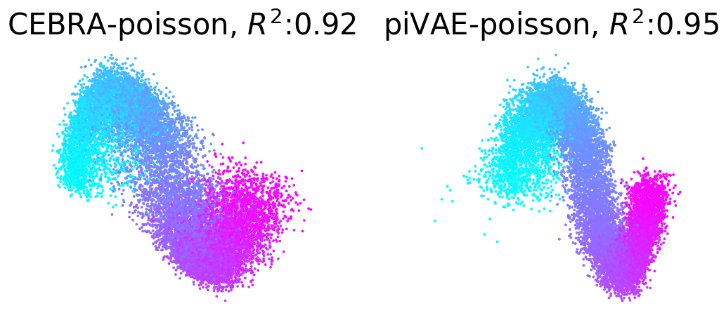
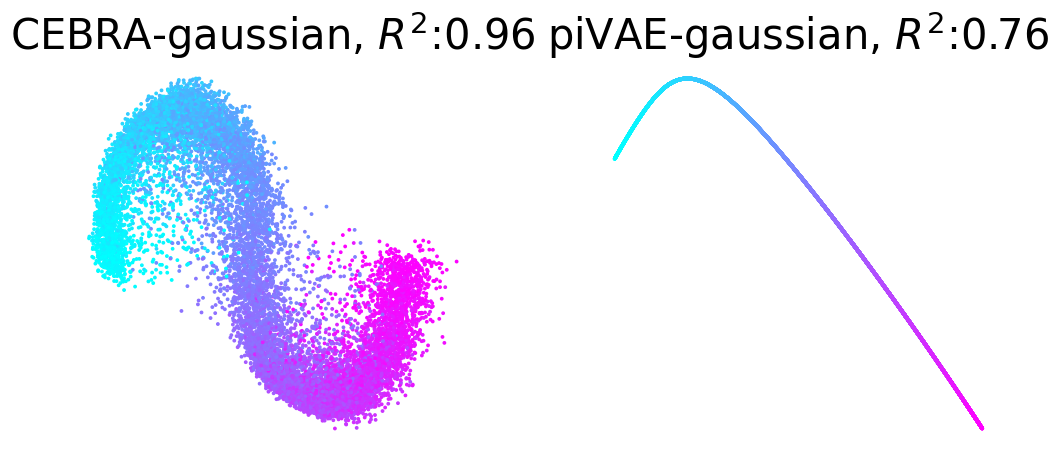
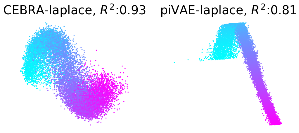
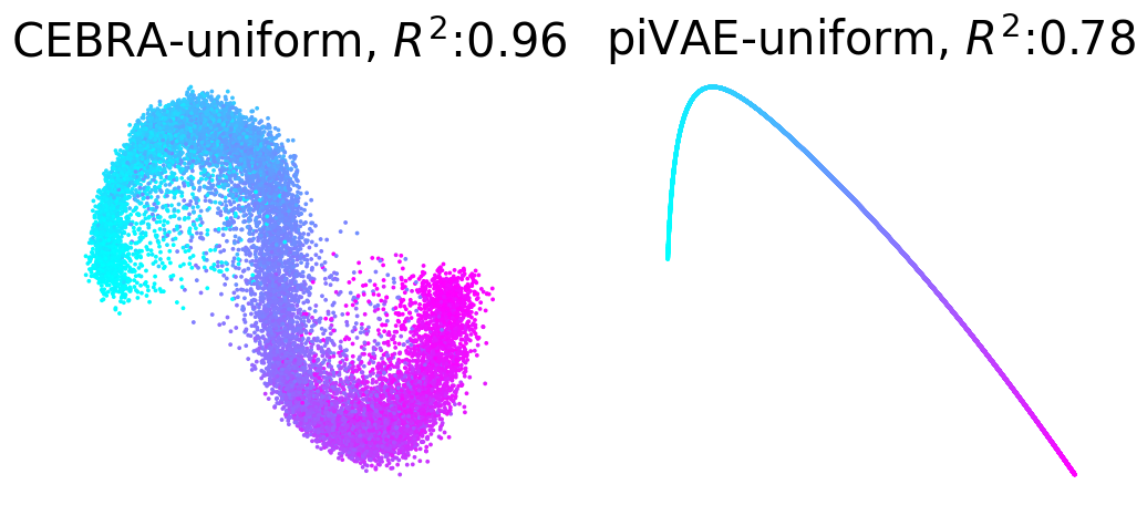
Plot example output embeddings from CEBRA (left) and piVAE (right) with R^2 scores#
For reference, here is the ground truth (left) and an example CEBRA embedding (right).

True 2D latent (Left). Each point is mapped to spiking rate of 100 neurons, and middle; CEBRA space embedding after linear regression to true latent. Reconstruction score of 100 seeds. Reconstruction score is \(R^2\) of linear regression between true latent and resulting embedding from each method. The behavior label is a 1D random variable sampled from uniform distribution of [0, \(2\pi\)] which is assigned to each time bin of synthetic neural data, visualized by the color map.
[12]:
pivae_embs = data["noise_exp_viz"]["pivae"]
cebra_embs = data["noise_exp_viz"]["cebra"]
label = data["noise_exp_viz"]["label"]
z = data["noise_exp_viz"]["z"]


def fitting(x, y):
    lin_model = sklearn.linear_model.LinearRegression()
    lin_model.fit(x, y)
    return lin_model.score(x, y), lin_model.predict(x)


emission_dict = {"pivae": {}, "cebra": {}}

for i, dist in enumerate(["poisson", "gaussian", "laplace", "uniform"]):
    pivae_emission = pivae_embs[dist]
    cebra_emission = cebra_embs[dist]
    cebra_score, fit_cebra = fitting(cebra_emission, z)
    pivae_score, fit_pivae = fitting(pivae_emission, z)
    fig = plt.figure(figsize=(12, 5))
    plt.subplots_adjust(wspace=0.3)
    ax = plt.subplot(121)
    ax.scatter(fit_cebra[:, 0], fit_cebra[:, 1], c=label, s=3, cmap="cool")
    ax.set_title(f"CEBRA-{dist}, $R^2$:{cebra_score:.2f}", fontsize=30)
    ax.axis("off")
    ax = plt.subplot(122)
    ax.scatter(fit_pivae[:, 0], fit_pivae[:, 1], c=label, s=3, cmap="cool")
    ax.set_title(f"piVAE-{dist}, $R^2$:{pivae_score:.2f}", fontsize=30)
    ax.axis("off")
    fig.savefig(f"emission_viz_{dist}.png", transparent=True, bbox_inches="tight")
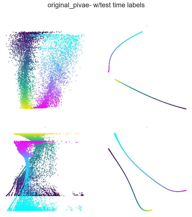
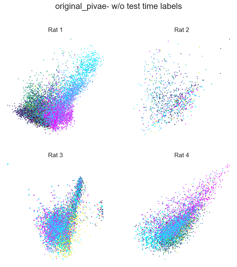
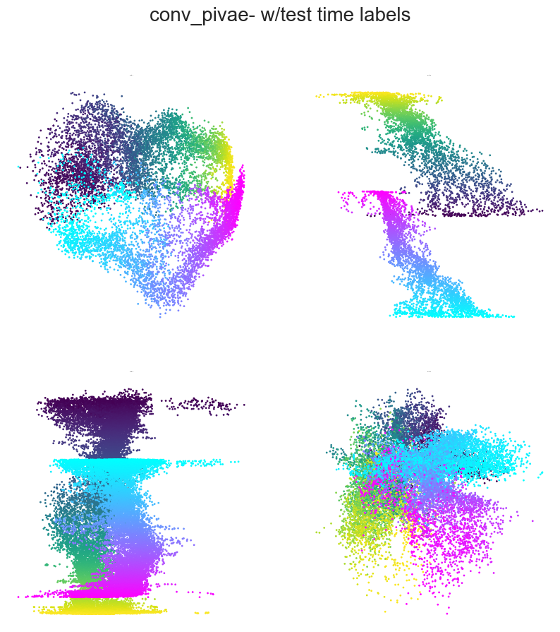
Plotting example embeddings from the original piVAE vs. our time-resolved conv-piVAE#
[13]:
for model in ["original_pivae", "conv_pivae"]:
    embs = data[model]

    sns.set_style("white")
    fig = plt.figure(figsize=(10, 10))
    plt.title(f"{model}- w/test time labels", fontsize=20, y=1.1)
    plt.subplots_adjust(wspace=0.2, hspace=0.2)
    plt.axis("off")
    ind1, ind2 = 0, 1

    for i in range(4):
        ax = fig.add_subplot(2, 2, i + 1)
        ax.set_title(f"Rat {i+1}", fontsize=1.5)
        plt.axis("off")
        emb = embs["w_label"]["embedding"][i]
        label = embs["w_label"]["label"][i]
        r_ind = label[:, 1] == 1
        l_ind = label[:, 2] == 1
        r = ax.scatter(
            emb[r_ind, ind1], emb[r_ind, ind2], s=1, c=label[r_ind, 0], cmap="viridis"
        )
        l = ax.scatter(
            emb[l_ind, ind1], emb[l_ind, ind2], s=1, c=label[l_ind, 0], cmap="cool"
        )

    fig = plt.figure(figsize=(10, 10))
    plt.title(f"{model}- w/o test time labels", fontsize=20, y=1.1)
    plt.subplots_adjust(wspace=0.2, hspace=0.2)
    plt.axis("off")
    for i in range(4):
        ax = fig.add_subplot(2, 2, i + 1)
        ax.set_title(f"Rat {i+1}", fontsize=15)
        plt.axis("off")
        emb = embs["wo_label"]["embedding"][i]
        label = embs["wo_label"]["label"][i]
        r_ind = label[:, 1] == 1
        l_ind = label[:, 2] == 1
        r = ax.scatter(
            emb[r_ind, ind1], emb[r_ind, ind2], s=1, c=label[r_ind, 0], cmap="viridis"
        )
        l = ax.scatter(
            emb[l_ind, ind1], emb[l_ind, ind2], s=1, c=label[l_ind, 0], cmap="cool"
        )

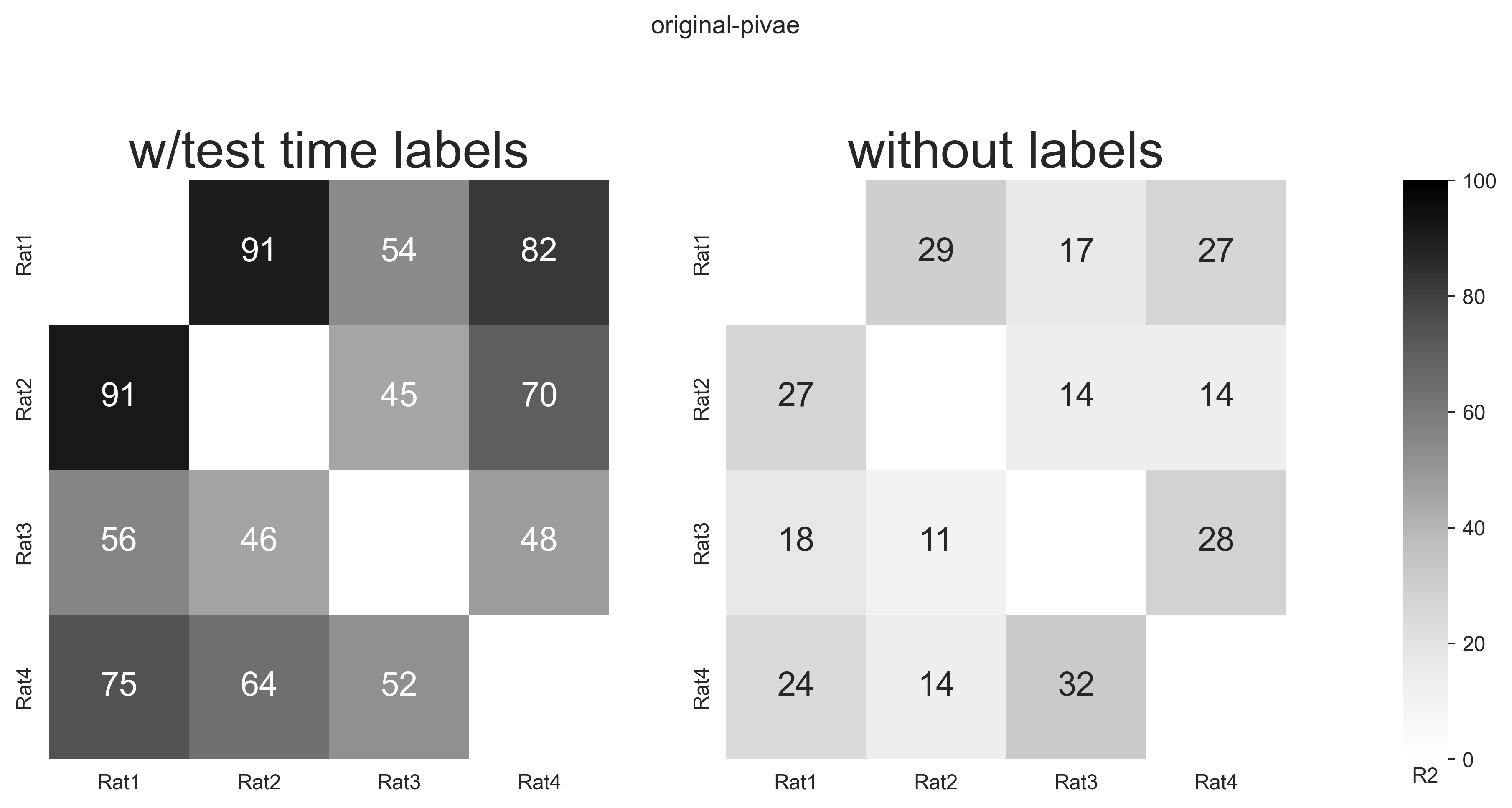
Plotting example embeddings from the original piVAE vs. our time-resolved conv-piVAE#
[14]:
methods_name = ["w/test time labels", "without labels"]
def prepare_heatmap(scores, n_item):
scores = scores.reshape(n_item, n_item - 1)
return np.array([np.insert(scores[i], i, None) for i in range(n_item)])
fig, axs = plt.subplots(
ncols=3,
nrows=1,
figsize=(12, 5),
gridspec_kw={"width_ratios": [1, 1, 0.08]},
dpi=360,
)
fig.suptitle("original-pivae", y=1.1)
subjects = ["Rat1", "Rat2", "Rat3", "Rat4"]
scores = [
data["original_pivae"]["w_label"]["consistency"],
data["original_pivae"]["wo_label"]["consistency"],
]
sns.set(font_scale=2.0)
for i, method in enumerate(methods_name):
score = prepare_heatmap(np.array(scores[i]), 4)
if i == 0:
hmap = sns.heatmap(
ax=axs[i],
data=score,
vmin=0.0,
vmax=100,
cmap=sns.color_palette("Greys", as_cmap=True),
annot=True,
xticklabels=subjects,
annot_kws={"fontsize": 16},
yticklabels=subjects,
cbar=False,
)
elif i == 1:
hmap = sns.heatmap(
ax=axs[i],
data=score,
vmin=0.0,
vmax=100,
cmap=sns.color_palette("Greys", as_cmap=True),
annot=True,
xticklabels=subjects,
annot_kws={"fontsize": 16},
yticklabels=subjects,
cbar_ax=axs[2],
)
hmap.set_title(method, fontsize=25)
plt.subplots_adjust(wspace=0.3)
axs[-1].set_xlabel("R2")
fig, axs = plt.subplots(
ncols=3,
nrows=1,
figsize=(12, 5),
gridspec_kw={"width_ratios": [1, 1, 0.08]},
dpi=360,
)
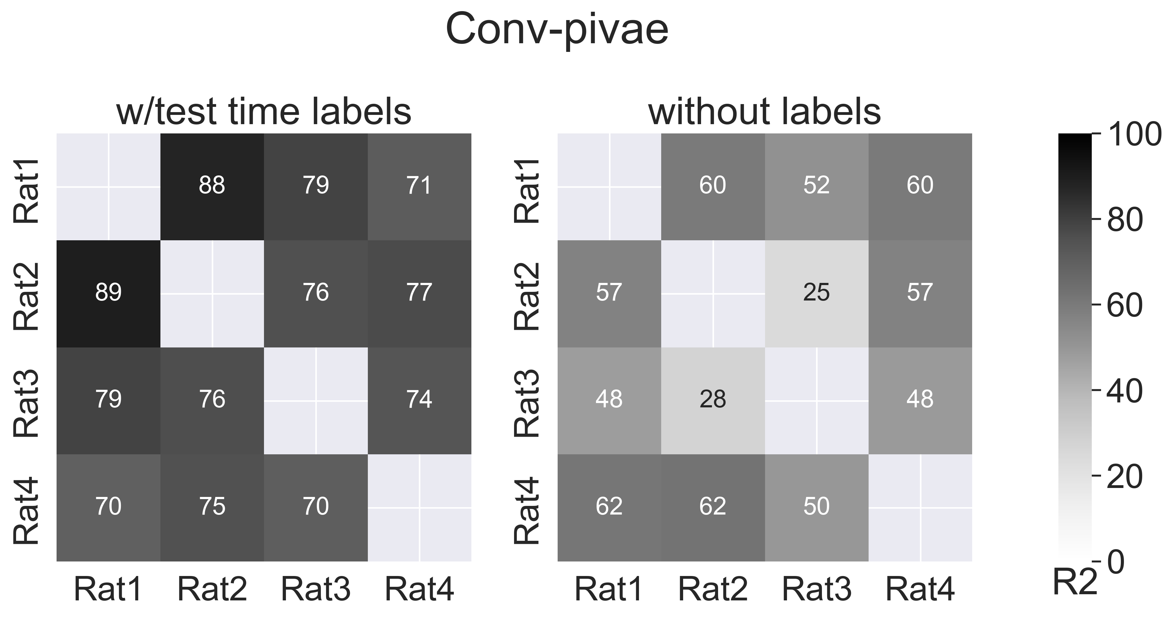
fig.suptitle("Conv-pivae", y=1.1)
subjects = ["Rat1", "Rat2", "Rat3", "Rat4"]
scores = [
data["conv_pivae"]["w_label"]["consistency"],
data["conv_pivae"]["wo_label"]["consistency"],
]
sns.set(font_scale=2.0)
for i, method in enumerate(methods_name):
score = prepare_heatmap(np.array(scores[i]), 4)
if i == 0:
hmap = sns.heatmap(
ax=axs[i],
data=score,
vmin=0.0,
vmax=100,
cmap=sns.color_palette("Greys", as_cmap=True),
annot=True,
xticklabels=subjects,
annot_kws={"fontsize": 16},
yticklabels=subjects,
cbar_ax=axs[2],
)
elif i == 1:
hmap = sns.heatmap(
ax=axs[i],
data=score,
vmin=0.0,
vmax=100,
cmap=sns.color_palette("Greys", as_cmap=True),
annot=True,
xticklabels=subjects,
annot_kws={"fontsize": 16},
yticklabels=subjects,
cbar_ax=axs[2],
)
hmap.set_title(method, fontsize=25)
plt.subplots_adjust(wspace=0.3)
axs[-1].set_xlabel("R2")
[14]:
Text(0.5, 177.99999999999997, 'R2')