You can download and run the notebook locally:

---

Figure 3: Forelimb movement behavior in a primate

For reference, here is the full figure

import plot and data loading dependencies

import numpy as np
import pandas as pd
import matplotlib.pyplot as plt
import seaborn as sns

data = pd.read_hdf("../data/Figure3.h5", key = "data")

Figure 3a

• Behavioral setup: monkey makes either active movements in 8 directions with the manipulandum, or the arm is passively moved via the manipulandum (real behavioral trajectories shown, with cartoon depicting the task setup). Behavior and neural recordings are from area 2 of the primary somatosensory cortex from Chowdhury et al.

active = data["behavior"]["active"]
active_target = data["behavior"]["active_target"]

passive = data["behavior"]["passive"]
passive_target = data["behavior"]["passive_target"]

fig = plt.figure(figsize=(8, 4))
ax1 = plt.subplot(121)
ax1.scatter(active[:, 0], active[:, 1], color=plt.cm.hsv(1 / 8 * active_target), s=1)
ax1.axis("off")

ax2 = plt.subplot(122)
ax2.scatter(passive[:, 0], passive[:, 1], color=plt.cm.hsv(1 / 8 * passive_target), s=1)
ax2.axis("off")

(-7.249750447273255, 6.267432045936585, -4.10022519826889, 3.132592189311981)

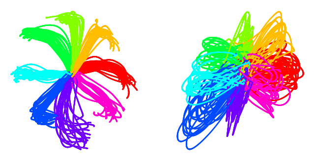
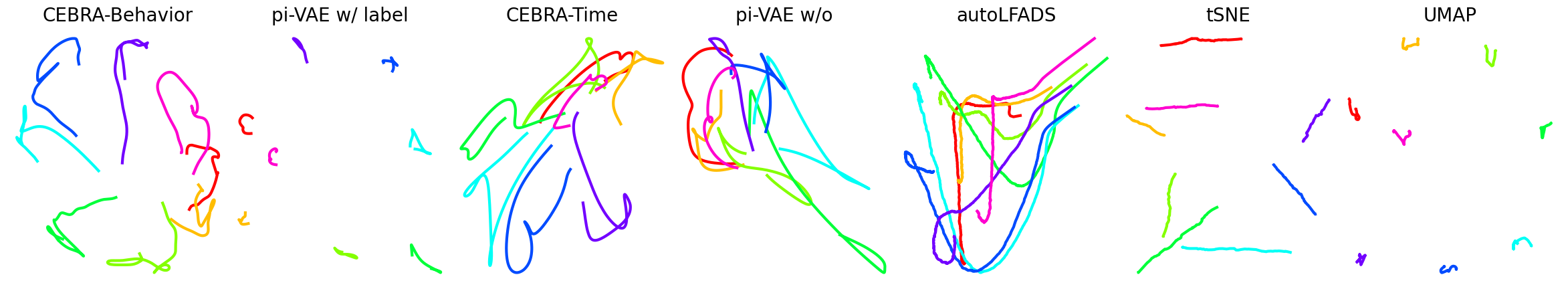
Figure 3b

• Comparison of embeddings of active trials generated with CEBRA-Behavior, CEBRA-Time, conv-pi-VAE variants, tSNE, and UMAP. The embeddings of trials (n=364) of each direction are post-hoc averaged.

overview = data["overview"]
fig = plt.figure(figsize=(30, 5))
plt.subplots_adjust(wspace=0, hspace=0)
emissions_list = [
    overview["cebra-behavior"],
    overview["pivae_w"],
    overview["cebra-time"],
    overview["pivae_wo"],
    overview["autolfads"],
    overview["tsne"],
    overview["umap"],
]
num_plots = len(emissions_list)
labels = overview["label"]

def plot_subplot(ax, j, lw = 2):

    if j == 0:
        idx1, idx2 = (2, 0)

    elif j == 1 or j == 3:
        idx1, idx2 = (2, 3)

    elif j == 5 or j == 6:
        idx1, idx2 = (0, 1)

    else:
        idx1, idx2 = (0, 1)


    if j == 0:
        trials = emissions_list[j].reshape(-1, 600, 4)
        trials_labels = labels.reshape(-1, 600)[:, 1]
        mean_trials = []
        for i in range(8):
            mean_trial = trials[trials_labels == i].mean(axis=0)
            mean_trials.append(mean_trial)
        for trial, label in zip(mean_trials, np.arange(8)):
            ax.plot(
                trial[:, idx1], trial[:, idx2], color=plt.cm.hsv(1 / 8 * label),
                linewidth = lw
            )
    elif j == 1:
        trials = emissions_list[j].reshape(-1, 600, 4)
        trials_labels = labels.reshape(-1, 600)[:, 1]
        mean_trials = []
        for i in range(8):
            mean_trial = trials[trials_labels == i].mean(axis=0)
            mean_trials.append(mean_trial)
        for trial, label in zip(mean_trials, np.arange(8)):
            ax.plot(
                trial[:, idx1], trial[:, idx2], color=plt.cm.hsv(1 / 8 * label),
              linewidth = lw
            )
    elif j == 4:
        mean_trials = emissions_list[j]
        for trial, label in zip(mean_trials, np.arange(8)):
            ax.plot(
                trial[:, idx1], trial[:, idx2], color=plt.cm.hsv(1 / 8 * label),
              linewidth = lw
            )
    else:
        trials = emissions_list[j].reshape(-1, 600, emissions_list[j].shape[-1])
        trials_labels = labels.reshape(-1, 600)[:, 1]
        mean_trials = []
        for i in range(8):
            mean_trial = trials[trials_labels == i].mean(axis=0)
            mean_trials.append(mean_trial)
        for trial, label in zip(mean_trials, np.arange(8)):
            ax.plot(
                trial[:, idx1], trial[:, idx2], color=plt.cm.hsv(1 / 8 * label),
              linewidth = lw
            )
    ax.spines["top"].set_visible(False)
    ax.spines["right"].set_visible(False)
    ax.spines["bottom"].set_visible(False)
    ax.spines["left"].set_visible(False)
    ax.set_xticks([])
    ax.set_yticks([])
    ax.set_title(
        [
            "CEBRA-Behavior",
            "pi-VAE w/ label",
            "CEBRA-Time",
            "pi-VAE w/o",
            "autoLFADS",
            "tSNE",
            "UMAP",
        ][j],
        fontsize=20,
    )
    return ax


for j in range(num_plots):
    if j == 0:
        idx1, idx2 = (2, 0)
        ax = fig.add_subplot(1, num_plots, j + 1)
    elif j == 1 or j == 3:
        idx1, idx2 = (2, 3)
        ax = fig.add_subplot(1, num_plots, j + 1)
    elif j == 5 or j == 6:
        idx1, idx2 = (0, 1)
        ax = fig.add_subplot(1, num_plots, j + 1)
    else:
        idx1, idx2 = (0, 1)
        ax = fig.add_subplot(1, num_plots, j + 1)
    plot_subplot(ax, j, lw = 3)
plt.show()

# Uncomment to generate high-quality plots of the paper

#for j in range(num_plots):
#  fig = plt.figure(figsize=(5, 5), dpi = 300)
#  ax = plot_subplot(plt.gca(), j, lw= 3)
#  ax.set_aspect("equal")
#  plt.savefig(f"monkey_{j}.svg", bbox_inches = "tight", transparent = True)
#  plt.show()

The embedding sizes of the various models can be obtained as follows (and the plot above adapted to show other dimensions). Note that autoLFADS was trained in 4D, and was then projected to 2D using a PCA.

methods = [
  "cebra-behavior",
  "pivae_w",
  "cebra-time",
  "pivae_wo",
  "autolfads",
  "tsne",
  "umap",
]

emissions_list = [
    overview["cebra-behavior"],
    overview["pivae_w"],
    overview["cebra-time"],
    overview["pivae_wo"],
    overview["tsne"],
    overview["umap"],
]

for m, e in zip(methods, emissions_list):
  print(m, e.shape)

cebra-behavior (115800, 4)
pivae_w (115800, 4)
cebra-time (115800, 4)
pivae_wo (115800, 4)
autolfads (115800, 2)
tsne (115800, 2)

Figure 3c

• CEBRA-Behavior trained with x,y position of the hand. Left panel is color-coded to x position and right panel is color-coded to y position.

def set_pane_axis(ax):
    ax.xaxis.set_pane_color((1.0, 1.0, 1.0, 0.0))
    ax.yaxis.set_pane_color((1.0, 1.0, 1.0, 0.0))
    ax.zaxis.set_pane_color((1.0, 1.0, 1.0, 0.0))
    ax.xaxis._axinfo["grid"]["color"] = (1, 1, 1, 0)
    ax.yaxis._axinfo["grid"]["color"] = (1, 1, 1, 0)
    ax.zaxis._axinfo["grid"]["color"] = (1, 1, 1, 0)
    ax.xaxis.set_ticks([])
    ax.yaxis.set_ticks([])
    ax.zaxis.set_ticks([])


features_pos = data["behavior_time"]["behavior"]["embedding"]
labels_pos = data["behavior_time"]["behavior"]["label"]
dx1, idx2, idx3 = (0, 1, 2)
fig = plt.figure(figsize=(12, 6))
fig.suptitle("CEBRA-Behavior, labels - continuous position", fontsize=20)
ax1 = fig.add_subplot(1, 2, 1, projection="3d")
ax1.set_title(f"x pos")
x = ax1.scatter(
    features_pos[:, idx1],
    features_pos[:, idx2],
    features_pos[:, idx3],
    cmap="seismic",
    c=labels_pos[:, 0],
    s=0.05,
    vmin=-15,
    vmax=15,
)

ax2 = fig.add_subplot(1, 2, 2, projection="3d")
ax2.set_title(f"y pos")
y = ax2.scatter(
    features_pos[:, idx1],
    features_pos[:, idx2],
    features_pos[:, idx3],
    cmap="seismic",
    c=labels_pos[:, 1],
    s=0.05,
    vmin=-15,
    vmax=15,
)
yc = plt.colorbar(y, fraction=0.03, pad=0.05, ticks=np.linspace(-15, 15, 7))
yc.ax.tick_params(labelsize=15)
yc.ax.set_title("(cm)", fontsize=10)
set_pane_axis(ax1)
set_pane_axis(ax2)

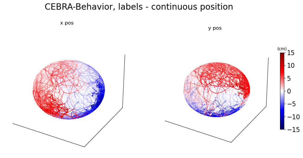
Figure 3d

• CEBRA-Time without any external behavior variables. As in \textbf{c}, left and right are color-coded to x and y position, respectively.

features_time = data["behavior_time"]["time"]["embedding"]
labels_time = data["behavior_time"]["time"]["label"]
idx1, idx2, idx3 = (0, 1, 2)
fig = plt.figure(figsize=(12, 6))
fig.suptitle("CEBRA-Time, labels - continuous position", fontsize=20)
ax1 = fig.add_subplot(1, 2, 1, projection="3d")
ax1.set_title(f"x pos")
x = ax1.scatter(
    features_time[:, idx1],
    features_time[:, idx2],
    features_time[:, idx3],
    cmap="seismic",
    c=labels_time[:, 0],
    s=0.05,
    vmin=-15,
    vmax=15,
)

ax2 = fig.add_subplot(1, 2, 2, projection="3d")
ax2.set_title(f"y pos")
y = ax2.scatter(
    features_time[:, idx1],
    features_time[:, idx2],
    features_time[:, idx3],
    cmap="seismic",
    c=labels_time[:, 1],
    s=0.05,
    vmin=-15,
    vmax=15,
)
yc = plt.colorbar(y, fraction=0.03, pad=0.05, ticks=np.linspace(-15, 15, 7))
yc.ax.tick_params(labelsize=15)
yc.ax.set_title("(cm)", fontsize=10)
set_pane_axis(ax1)
set_pane_axis(ax2)

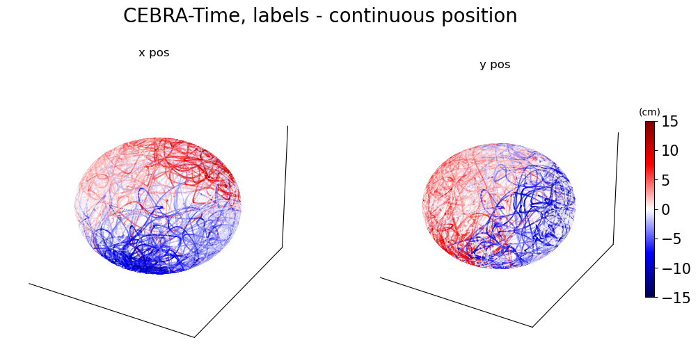
Figure 3e

• Left, CEBRA-Behavior embedding trained with a 4D latent space, with target direction and active OR passive trials (trained separately) as behavior labels. Plotted separately, active vs. passive training condition.

active_emission = data["cebra_ap_sep"]["active"]["embedding"]
active_label = data["cebra_ap_sep"]["active"]["label"]
passive_emission = data["cebra_ap_sep"]["passive"]["embedding"]
passive_label = data["cebra_ap_sep"]["passive"]["label"]
feature_num = active_emission.shape[-1]

fig = plt.figure(
    figsize=(20, 10),
)
fig.suptitle(
    "Separately trained active/passive trials with direction (1-8) labels", fontsize=20
)
idx1, idx2, idx3 = 1, 2, 0
active_trials_index = active_label

active_trials = active_emission.reshape(-1, 600, feature_num)
active_trials_labels = active_label.reshape(-1, 600)[:, 0].squeeze()
mean_active_trials = []

for i in range(8):
    mean_active_trial = active_trials[active_trials_labels == i].mean(
        axis=0
    ) / np.linalg.norm(active_trials[active_trials_labels == i].mean(axis=0))
    mean_active_trials.append(mean_active_trial)

ax1 = fig.add_subplot(1, 2, 1, projection="3d")
for trial, label in zip(mean_active_trials, np.arange(8)):
    ax1.plot(
        trial[:, idx1], trial[:, idx2], trial[:, idx3], color=plt.cm.hsv(1 / 8 * label)
    )
    ax1.plot(
        trial[0, idx1],
        trial[0, idx2],
        trial[0, idx3],
        color=plt.cm.hsv(1 / 8 * label),
        marker="o",
        markersize=10,
    )
    ax1.plot(
        trial[-1, idx1],
        trial[-1, idx2],
        trial[-1, idx3],
        color=plt.cm.hsv(1 / 8 * label),
        marker="<",
        markersize=10,
    )
set_pane_axis(ax1)
ax1.set_title("Active", fontsize=20)


passive_trials_index = passive_label
passive_trials = passive_emission.reshape(-1, 600, feature_num)
passive_trials_labels = passive_label.reshape(-1, 600)[:, 0].squeeze()
mean_passive_trials = []

for i in range(8):
    mean_passive_trial = passive_trials[passive_trials_labels == i].mean(
        axis=0
    ) / np.linalg.norm(passive_trials[passive_trials_labels == i].mean(axis=0))
    mean_passive_trials.append(mean_passive_trial)

ax2 = fig.add_subplot(1, 2, 2, projection="3d")
for trial, label in zip(mean_passive_trials, np.arange(8)):
    ax2.plot(
        trial[:, idx1], trial[:, idx2], trial[:, idx3], color=plt.cm.hsv(1 / 8 * label)
    )
    ax2.plot(
        trial[0, idx1],
        trial[0, idx2],
        trial[0, idx3],
        color=plt.cm.hsv(1 / 8 * label),
        marker="o",
        markersize=10,
    )
    ax2.plot(
        trial[-1, idx1],
        trial[-1, idx2],
        trial[-1, idx3],
        color=plt.cm.hsv(1 / 8 * label),
        marker="<",
        markersize=10,
    )
set_pane_axis(ax2)
ax2.set_title("Passive", fontsize=20)

Text(0.5, 0.92, 'Passive')

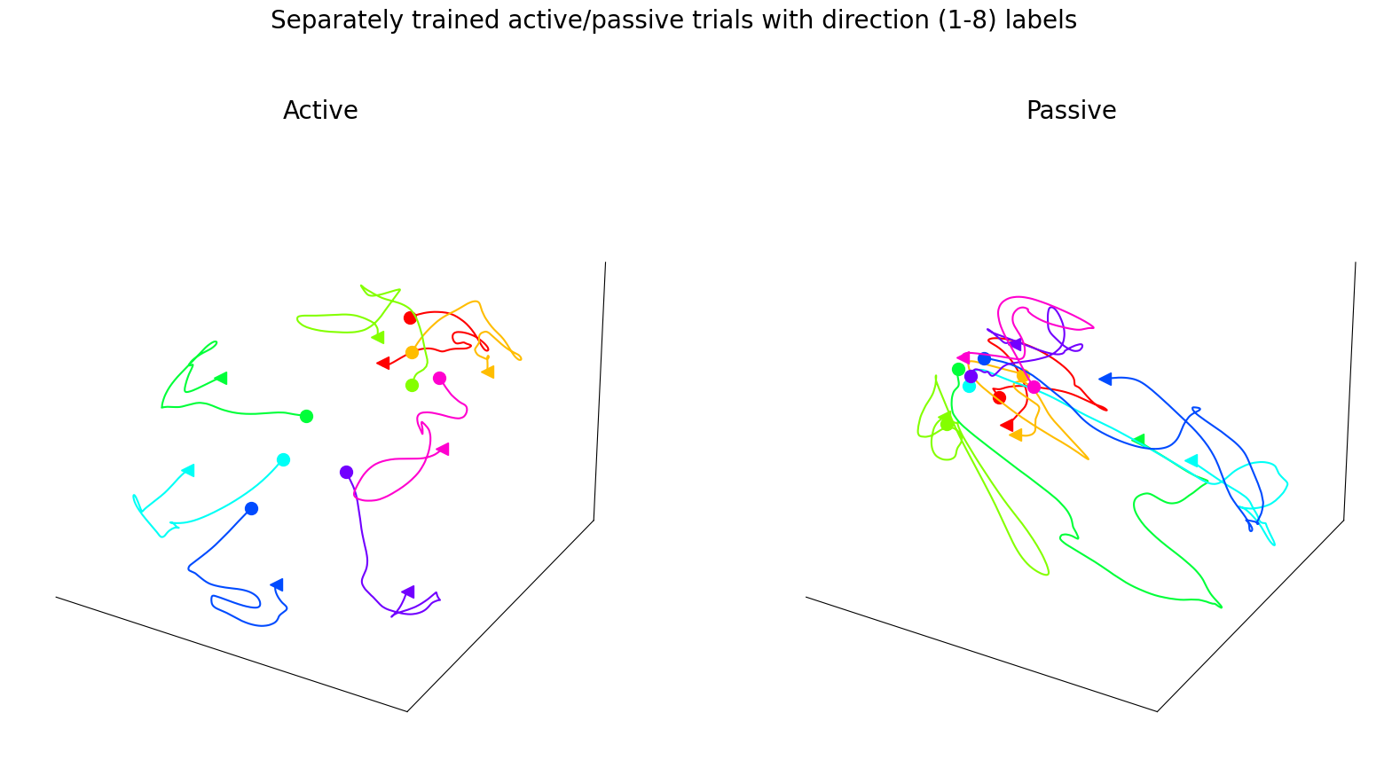
Figure 3f

• Left, CEBRA-Behavior embedding trained with a 4D latent space, with target direction and active and passive trials as behavior labels, but plotted separately, active vs. passive trials.

target_emission = data["cebra_ap_all"]["embedding"]
target_label = data["cebra_ap_all"]["label"]

fig = plt.figure(
    figsize=(20, 10),
)
fig.suptitle(
    "Concurrently trained active/passive trials with direction (1-8) + active/passive trial info labels",
    fontsize=20,
)
idx1, idx2, idx3 = 2, 0, 1
active_trials_index = target_label < 8
active_trials = target_emission[active_trials_index].reshape(-1, 600, feature_num)
active_trials_labels = (
    target_label[active_trials_index].reshape(-1, 600)[:, 0].squeeze()
)
mean_active_trials = []

for i in range(8):
    mean_active_trial = (
        active_trials[active_trials_labels == i].mean(axis=0)
        / np.linalg.norm(active_trials[active_trials_labels == i].mean(axis=0), axis=1)[
            :, None
        ]
    )
    mean_active_trials.append(mean_active_trial)

ax1 = fig.add_subplot(1, 2, 1, projection="3d")
for trial, label in zip(mean_active_trials, np.arange(8)):
    ax1.plot(
        trial[:, idx1], trial[:, idx2], trial[:, idx3], color=plt.cm.hsv(1 / 8 * label)
    )
    ax1.plot(
        trial[0, idx1],
        trial[0, idx2],
        trial[0, idx3],
        color=plt.cm.hsv(1 / 8 * label),
        marker="o",
        markersize=10,
    )
    ax1.plot(
        trial[-1, idx1],
        trial[-1, idx2],
        trial[-1, idx3],
        color=plt.cm.hsv(1 / 8 * label),
        marker="<",
        markersize=10,
    )
set_pane_axis(ax1)
ax1.set_title("Active", fontsize=20)

# ax3 = fig.add_subplot(2,2,3)
passive_trials_index = target_label >= 8
passive_trials = target_emission[passive_trials_index].reshape(-1, 600, feature_num)
passive_trials_labels = (
    target_label[passive_trials_index].reshape(-1, 600)[:, 0].squeeze()
)
mean_passive_trials = []

for i in range(8, 16):
    mean_passive_trial = (
        passive_trials[passive_trials_labels == i].mean(axis=0)
        / np.linalg.norm(
            passive_trials[passive_trials_labels == i].mean(axis=0), axis=1
        )[:, None]
    )
    mean_passive_trials.append(mean_passive_trial)

ax2 = fig.add_subplot(1, 2, 2, projection="3d")

for trial, label in zip(mean_passive_trials, np.arange(8, 16)):
    ax2.plot(
        trial[:, idx1],
        trial[:, idx2],
        trial[:, idx3],
        color=plt.cm.hsv(1 / 8 * (label - 8)),
    )
    ax2.plot(
        trial[0, idx1],
        trial[0, idx2],
        trial[0, idx3],
        color=plt.cm.hsv(1 / 8 * (label - 8)),
        marker="o",
        markersize=10,
    )
    ax2.plot(
        trial[-1, idx1],
        trial[-1, idx2],
        trial[-1, idx3],
        color=plt.cm.hsv(1 / 8 * (label - 8)),
        marker="<",
        markersize=10,
    )
set_pane_axis(ax2)
ax2.set_title("Passive", fontsize=20)

Text(0.5, 0.92, 'Passive')

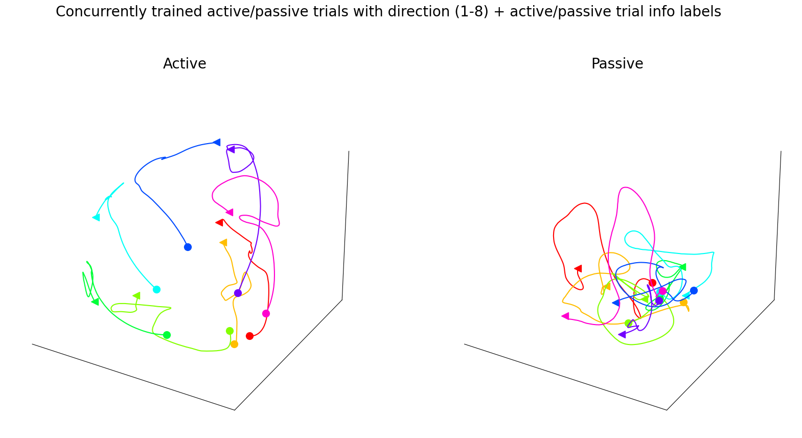
Figure 3g

• CEBRA-Behavior embedding trained with a 4D latent space using active and passive trials with continuous position as behavior labels, but post-hoc plotted separately, active vs. passive trials. The trajectory of each direction is averaged across trials (n=18–30 each, per directions) over time. Each trajectory represents 600ms from -100ms before the start of the movement.

position_emission = data["cebra_pos"]["embedding"]

fig = plt.figure(
    figsize=(20, 10),
)
fig.suptitle("Trained with continuous position label", fontsize=20)

idx1, idx2, idx3 = 0, 1, 2
active_trials_index = target_label < 8

active_trials = position_emission[active_trials_index].reshape(-1, 600, feature_num)
ctive_trials_labels = target_label[active_trials_index].reshape(-1, 600)[:, 0].squeeze()
mean_active_trials = []

for i in range(8):
    mean_active_trial = (
        active_trials[active_trials_labels == i].mean(axis=0)
        / np.linalg.norm(active_trials[active_trials_labels == i].mean(axis=0), axis=1)[
            :, None
        ]
    )
    mean_active_trials.append(mean_active_trial)

ax1 = fig.add_subplot(1, 2, 1, projection="3d")
for trial, label in zip(mean_active_trials, np.arange(8)):
    ax1.plot(
        trial[:, idx1], trial[:, idx2], trial[:, idx3], color=plt.cm.hsv(1 / 8 * label)
    )
    ax1.plot(
        trial[0, idx1],
        trial[0, idx2],
        trial[0, idx3],
        color=plt.cm.hsv(1 / 8 * label),
        marker="o",
        markersize=10,
    )
    ax1.plot(
        trial[-1, idx1],
        trial[-1, idx2],
        trial[-1, idx3],
        color=plt.cm.hsv(1 / 8 * label),
        marker="<",
        markersize=10,
    )
set_pane_axis(ax1)
ax1.set_title("Active", fontsize=20)

passive_trials_index = target_label >= 8
passive_trials = position_emission[passive_trials_index].reshape(-1, 600, feature_num)
passive_trials_labels = (
    target_label[passive_trials_index].reshape(-1, 600)[:, 0].squeeze()
)
mean_passive_trials = []

for i in range(8, 16):
    mean_passive_trial = (
        passive_trials[passive_trials_labels == i].mean(axis=0)
        / np.linalg.norm(
            passive_trials[passive_trials_labels == i].mean(axis=0), axis=1
        )[:, None]
    )
    mean_passive_trials.append(mean_passive_trial)

ax2 = fig.add_subplot(1, 2, 2, projection="3d")

for trial, label in zip(mean_passive_trials, np.arange(8, 16)):
    ax2.plot(
        trial[:, idx1],
        trial[:, idx2],
        trial[:, idx3],
        color=plt.cm.hsv(1 / 8 * (label - 8)),
    )
    ax2.plot(
        trial[0, idx1],
        trial[0, idx2],
        trial[0, idx3],
        color=plt.cm.hsv(1 / 8 * (label - 8)),
        marker="o",
        markersize=10,
    )
    ax2.plot(
        trial[-1, idx1],
        trial[-1, idx2],
        trial[-1, idx3],
        color=plt.cm.hsv(1 / 8 * (label - 8)),
        marker="<",
        markersize=10,
    )
set_pane_axis(ax2)
ax2.set_title("Passive", fontsize=20)

Text(0.5, 0.92, 'Passive')

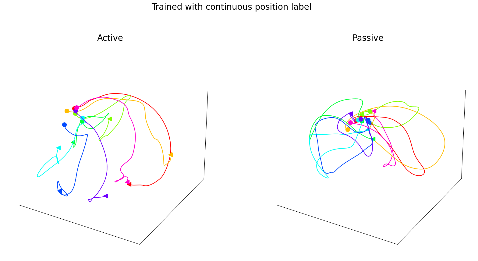
Figure 3h

• Left to right: Decoding performance of: position using CEBRA-Behavior trained with x,y position (active trials); target direction using CEBRA-Behavior trained with target direction (active trials); or active vs. passive accuracy using CEBRA-Behavior trained with both active and passive movements. For each case, we trained and evaluated 5 seeds represented by black dot and the orange line represents median.

position_acc = data["condition_decoding"]["position"]
direction_acc = data["condition_decoding"]["direction"]
ap_acc = data["condition_decoding"]["ap"]

sns.set(font_scale=3)
sns.set_style(
    "whitegrid",
    {"axes.grid": False},
)
fig = plt.figure(figsize=(5, 20))
axs = fig.subplots(3, 1)
plt.subplots_adjust(hspace=0.8)
data_list = [position_acc, direction_acc, ap_acc]
title_list = [
    "Position decoding (active)",
    "Direction decoding (active)",
    "AP decoding",
]

units = ["$R^2$ (%)", "Acc(%)", "Acc(%)"]
ylims = [(50, 100), (50, 80), (50, 100)]
for i in range(3):
    m = 0
    ax = sns.stripplot(
        data=[data_list[i][n] for n in ["3", "4", "8", "16", "32"]],
        facecolor="none",
        color="k",
        marker="$\circ$",
        s=10,
        jitter=0,
        ax=axs[i],
    )
    sns.boxplot(
        showmeans=False,
        medianprops={"color": "orange", "ls": "-", "lw": 2},
        whiskerprops={"visible": False},
        zorder=10,
        data=[data_list[i][n] for n in ["3", "4", "8", "16", "32"]],
        showfliers=False,
        showbox=False,
        showcaps=False,
        ax=axs[i],
    )

    ax.set_xlabel("Dimensions")
    ax.set_ylim(ylims[i])
    ax.set_ylabel(units[i])
    ax.set_title(title_list[i], y=1.1)
    ax.set_xticks(ticks=np.arange(5))
    ax.set_xticklabels(labels=[3, 4, 8, 16, 32])
    ax.spines["right"].set_visible(False)
    ax.spines["top"].set_visible(False)
plt.show()

/usr/lib/python3.10/site-packages/seaborn/categorical.py:166: FutureWarning: Setting a gradient palette using color= is deprecated and will be removed in version 0.13. Set `palette='dark:k'` for same effect.
  warnings.warn(msg, FutureWarning)
/usr/lib/python3.10/site-packages/seaborn/categorical.py:166: FutureWarning: Setting a gradient palette using color= is deprecated and will be removed in version 0.13. Set `palette='dark:k'` for same effect.
  warnings.warn(msg, FutureWarning)
/usr/lib/python3.10/site-packages/seaborn/categorical.py:166: FutureWarning: Setting a gradient palette using color= is deprecated and will be removed in version 0.13. Set `palette='dark:k'` for same effect.
  warnings.warn(msg, FutureWarning)

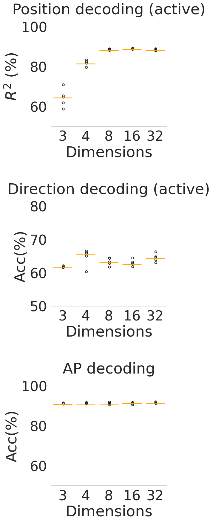
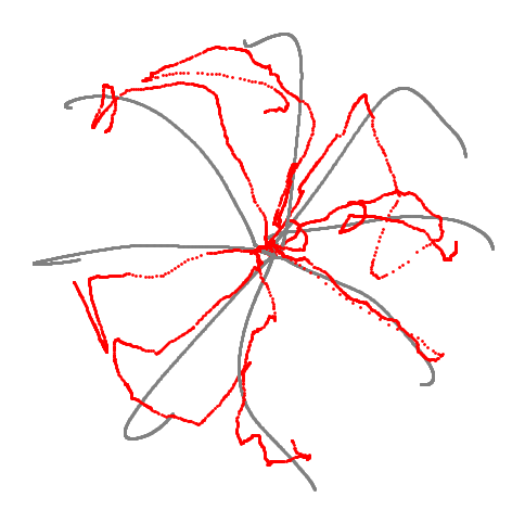
Figure 3i

• Decoded trajectory of hand position using CEBRA-Behavior trained on active trial with x,y position of hand. Grey line is true trajectory and red line is decoded trajectory.

true = data["trajectory"]["true"]
pred = data["trajectory"]["prediction"]
plt.figure(figsize=(6, 6))
for i in range(8):
    plt.scatter(true[i][:, 0], true[i][:, 1], s=1, c="gray")
    plt.scatter(pred[i][:, 0], pred[i][:, 1], s=1, c="red")
plt.axis("off")

(-13.162386083602906,
 12.013674879074097,
 -12.53279776573181,
 10.802085828781127)