You can download and run the notebook locally:

---

Extended Data Figure 8: Somatosensory cortex decoding from primate recording

import plot and data loading dependencies

import numpy as np
import matplotlib.pyplot as plt
import scipy.signal
import joblib as jl
import pandas as pd
import seaborn as sns

from matplotlib.lines import Line2D
from matplotlib import cm, colors

data = pd.read_hdf("../data/EDFigure8.h5")

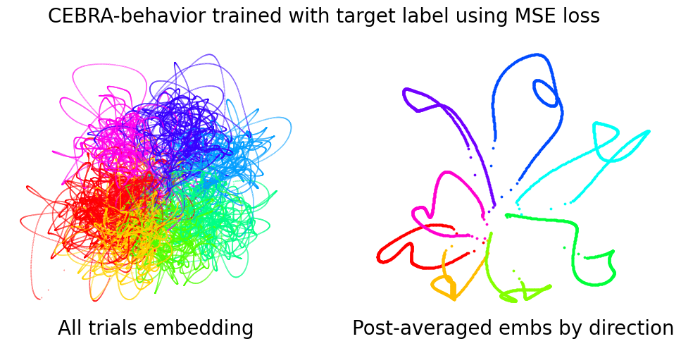
CEBRA models with MSE models on primate data

• As in Fig.3b, the embeddings of trials (n=364) of each direction are post-hoc averaged. Left is reproduced from Fig. 3b –CEBRA-Behavior, and right is CEBRA-Behavior trained with an added MSE loss.

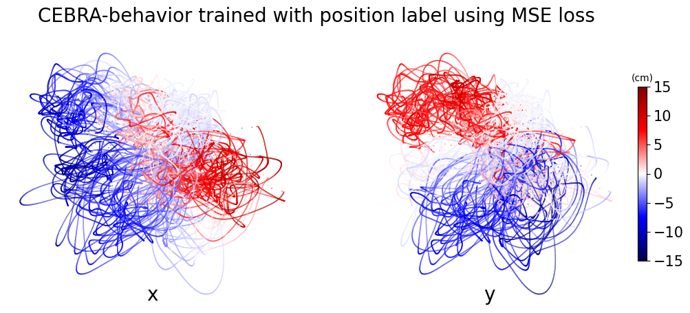
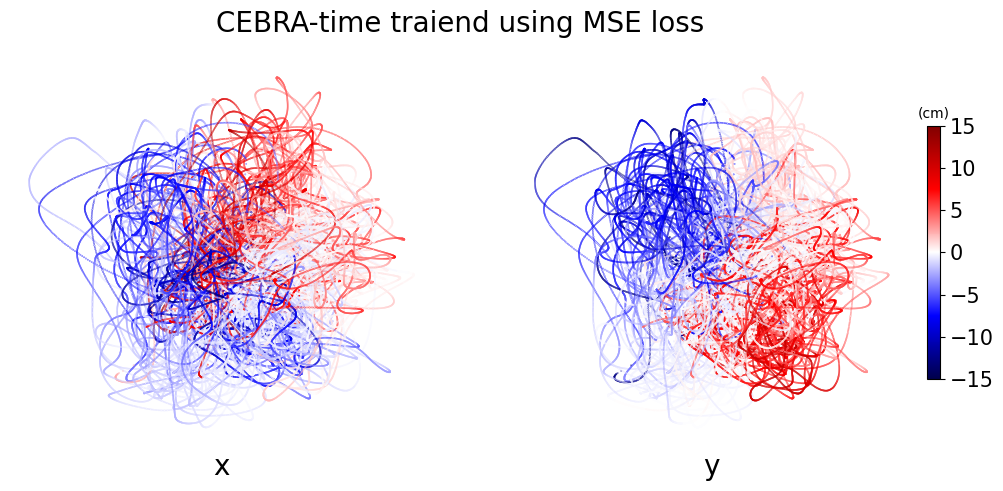
• CEBRA-Behavior trained with x,y position of the hand. Left panel is color-coded to x position and right panel is color-coded to y position.

cebra_target = data["monkey_mse_viz"]["cebra_target"]["emission"]
target_label = data["monkey_mse_viz"]["cebra_target"]["label"]
cebra_pos = data["monkey_mse_viz"]["cebra_pos"]["emission"]
pos_label = data["monkey_mse_viz"]["cebra_pos"]["label"]
cebra_time = data["monkey_mse_viz"]["cebra_time"]["emission"]


fig = plt.figure(figsize=(12, 5))
plt.suptitle("CEBRA-behavior trained with target label using MSE loss", fontsize=20)
ax = plt.subplot(121)
ax.set_title("All trials embedding", fontsize=20, y=-0.1)
x = ax.scatter(
    cebra_target[:, 0], cebra_target[:, 1], c=target_label, cmap=plt.cm.hsv, s=0.05
)
ax.axis("off")
ax = plt.subplot(122)
ax.set_title("Post-averaged embs by direction", fontsize=20, y=-0.1)
for i in range(8):
    direction_trial = target_label == i
    trial_avg = cebra_target[direction_trial, :].reshape(-1, 600, 2).mean(axis=0)
    ax.scatter(trial_avg[:, 0], trial_avg[:, 1], color=plt.cm.hsv(1 / 8 * i), s=3)
ax.axis("off")

fig = plt.figure(figsize=(12, 5))
plt.suptitle("CEBRA-behavior trained with position label using MSE loss", fontsize=20)
ax = plt.subplot(121)
ax.set_title("x", fontsize=20, y=0)
x = ax.scatter(
    cebra_pos[:, 0],
    cebra_pos[:, 1],
    c=pos_label[:, 0],
    cmap="seismic",
    s=0.05,
    vmin=-15,
    vmax=15,
)
ax.axis("off")
ax = plt.subplot(122)
y = ax.scatter(
    cebra_pos[:, 0],
    cebra_pos[:, 1],
    c=pos_label[:, 1],
    cmap="seismic",
    s=0.05,
    vmin=-15,
    vmax=15,
)
ax.axis("off")
ax.set_title("y", fontsize=20, y=0)
yc = plt.colorbar(y, fraction=0.03, pad=0.05, ticks=np.linspace(-15, 15, 7))
yc.ax.tick_params(labelsize=15)
yc.ax.set_title("(cm)", fontsize=10)

fig = plt.figure(figsize=(12, 5))
plt.suptitle("CEBRA-time traiend using MSE loss", fontsize=20)
ax = plt.subplot(121)
ax.set_title("x", fontsize=20, y=-0.1)
x = ax.scatter(
    cebra_time[:, 0],
    cebra_time[:, 1],
    c=pos_label[:, 0],
    cmap="seismic",
    s=0.05,
    vmin=-15,
    vmax=15,
)
ax.axis("off")
ax = plt.subplot(122)
y = ax.scatter(
    cebra_time[:, 0],
    cebra_time[:, 1],
    c=pos_label[:, 1],
    cmap="seismic",
    s=0.05,
    vmin=-15,
    vmax=15,
)
ax.axis("off")
ax.set_title("y", fontsize=20, y=-0.1)
yc = plt.colorbar(y, fraction=0.03, pad=0.05, ticks=np.linspace(-15, 15, 7))
yc.ax.tick_params(labelsize=15)
yc.ax.set_title("(cm)", fontsize=10)

Text(0.5, 1.0, '(cm)')

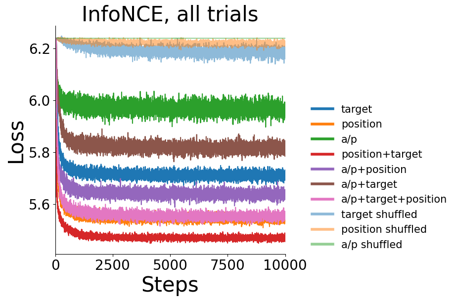
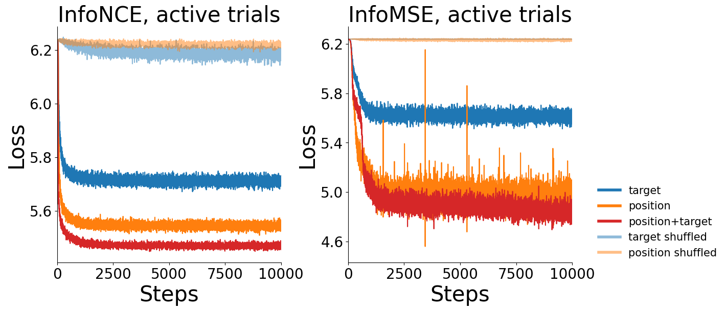
Loss (InfoNCE) vs. training iteration for CEBRA-Behavior with position, direction, active or passive, and position+direction labels (and shuffled labels, which show a lack of training) for all trials (left) or only active trials (right), or active trials with a MSE loss.

fig = plt.figure(figsize=(6, 6))
ax1 = fig.add_subplot(111)
ax1.set_title("InfoNCE, all trials", fontsize=30)
ax1.spines["top"].set_visible(False)
ax1.spines["right"].set_visible(False)

all_loss_data = data["all_trial_loss"]
all_ap = all_loss_data["ap"]
all_pos = all_loss_data["pos"]
all_target = all_loss_data["target"]
all_postarget = all_loss_data["pos_target"]
all_appos = all_loss_data["ap_pos"]
all_aptarget = all_loss_data["ap_target"]
all_appostarget = all_loss_data["ap_pos_target"]

all_ap_sh = all_loss_data["ap_shuffle"]
all_pos_sh = all_loss_data["pos_shuffle"]
all_target_sh = all_loss_data["target_shuffle"]

w = 9
p = 7


ax1.plot(scipy.signal.savgol_filter(all_target, w, p), label="target")
ax1.plot(
    scipy.signal.savgol_filter(all_pos, w, p),
    label="position",
)
ax1.plot(scipy.signal.savgol_filter(all_ap, w, p), label="a/p")

ax1.plot(
    scipy.signal.savgol_filter(all_target_sh, w, p),
    label="target shuffled",
    c=plt.cm.tab10(0),
    alpha=0.5,
)
ax1.plot(
    scipy.signal.savgol_filter(all_pos_sh, w, p),
    label="position shuffled",
    c=plt.cm.tab10(1),
    alpha=0.5,
)
ax1.plot(
    scipy.signal.savgol_filter(all_ap_sh, w, p),
    label="a/p shuffled",
    c=plt.cm.tab10(2),
    alpha=0.5,
)

ax1.plot(scipy.signal.savgol_filter(all_postarget, w, p), label="pos+target")
ax1.plot(scipy.signal.savgol_filter(all_appos, w, p), label="ap+pos")
ax1.plot(scipy.signal.savgol_filter(all_aptarget, w, p), label="ap+target")
ax1.plot(scipy.signal.savgol_filter(all_appostarget, w, p), label="ap+pos+target")

plt.xlim([0, 10000])
plt.xlabel("Steps", fontsize=30)
plt.xticks(np.linspace(0, 10000, 5), fontsize=20)
plt.yticks(np.linspace(6.2, 5.6, 4), fontsize=20)
plt.ylabel("Loss", fontsize=30)


custom_lines = [
    Line2D([0], [0], lw=4, c=plt.cm.tab10(0)),
    Line2D([0], [0], lw=4, c=plt.cm.tab10(1)),
    Line2D([0], [0], lw=4, c=plt.cm.tab10(2)),
    Line2D([0], [0], lw=4, c=plt.cm.tab10(3)),
    Line2D([0], [0], lw=4, c=plt.cm.tab10(4)),
    Line2D([0], [0], lw=4, c=plt.cm.tab10(5)),
    Line2D([0], [0], lw=4, c=plt.cm.tab10(6)),
    Line2D([0], [0], lw=4, c=plt.cm.tab10(0), alpha=0.5),
    Line2D([0], [0], lw=4, c=plt.cm.tab10(1), alpha=0.5),
    Line2D([0], [0], lw=4, c=plt.cm.tab10(2), alpha=0.5),
]
ax1.legend(
    custom_lines,
    [
        "target",
        "position",
        "a/p",
        "position+target",
        "a/p+position",
        "a/p+target",
        "a/p+target+position",
        "target shuffled",
        "position shuffled",
        "a/p shuffled",
    ],
    loc=(1.1, 0),
    frameon=False,
    fontsize=15,
)


fig = plt.figure(figsize=(13, 6))
plt.subplots_adjust(wspace=0.3)

ax2 = fig.add_subplot(121)
ax2.set_title("InfoNCE, active trials", fontsize=30)
ax2.spines["top"].set_visible(False)
ax2.spines["right"].set_visible(False)

w = 9
p = 7


active_nce_data = data["active_trial_loss"]
active_pos = active_nce_data["pos"]
active_target = active_nce_data["target"]
active_postarget = active_nce_data["pos_target"]

active_pos_sh = active_nce_data["pos_shuffle"]
active_target_sh = active_nce_data["target_shuffle"]

c_id = np.linspace(50, 250, 7, dtype=int)

ax2.plot(
    scipy.signal.savgol_filter(active_target, w, p), label="target", c=plt.cm.tab10(0)
)

ax2.plot(
    scipy.signal.savgol_filter(active_target_sh, w, p),
    label="target-shuffled",
    c=plt.cm.tab10(0),
    alpha=0.5,
)

ax2.plot(
    scipy.signal.savgol_filter(active_pos, w, p), label="position", c=plt.cm.tab10(1)
)
ax2.plot(
    scipy.signal.savgol_filter(active_pos_sh, w, p),
    label="position-shuffled",
    c=plt.cm.tab10(1),
    alpha=0.5,
)
ax2.plot(
    scipy.signal.savgol_filter(active_postarget, w, p),
    label="position+target",
    c=plt.cm.tab10(3),
)

plt.xlim([0, 10000])
plt.xlabel("Steps", fontsize=30)
plt.xticks(np.linspace(0, 10000, 5), fontsize=20)
plt.yticks(np.linspace(6.2, 5.6, 4), fontsize=20)
plt.ylabel("Loss", fontsize=30)


ax3 = fig.add_subplot(122)
ax3.set_title("InfoMSE, active trials", fontsize=30)
ax3.spines["top"].set_visible(False)
ax3.spines["right"].set_visible(False)

active_mse_data = data["active_mse_loss"]
active_pos = active_mse_data["pos"]
active_target = active_mse_data["target"]
active_postarget = active_mse_data["pos_target"]

active_pos_sh = active_mse_data["pos_shuffled"]
active_target_sh = active_mse_data["target_shuffled"]

c_id = np.linspace(50, 250, 7, dtype=int)

ax3.plot(
    scipy.signal.savgol_filter(active_target, w, p), label="target", c=plt.cm.tab10(0)
)

ax3.plot(
    scipy.signal.savgol_filter(active_target_sh, w, p),
    label="target-shuffled",
    c=plt.cm.tab10(0),
    alpha=0.5,
)

ax3.plot(
    scipy.signal.savgol_filter(active_pos, w, p), label="position", c=plt.cm.tab10(1)
)
ax3.plot(
    scipy.signal.savgol_filter(active_pos_sh, w, p),
    label="position-shuffled",
    c=plt.cm.tab10(1),
    alpha=0.5,
)
ax3.plot(
    scipy.signal.savgol_filter(active_postarget, w, p),
    label="position+target",
    c=plt.cm.tab10(3),
)


plt.legend(fontsize="large", loc=[1, 0])
plt.xlim([0, 10000])
plt.xlabel("Steps", fontsize=30)
plt.ylabel("Loss", fontsize=30)

custom_lines = [
    Line2D([0], [0], lw=4, c=plt.cm.tab10(0)),
    Line2D([0], [0], lw=4, c=plt.cm.tab10(1)),
    Line2D([0], [0], lw=4, c=plt.cm.tab10(3)),
    Line2D([0], [0], lw=4, c=plt.cm.tab10(0), alpha=0.5),
    Line2D([0], [0], lw=4, c=plt.cm.tab10(1), alpha=0.5),
]
ax3.legend(
    custom_lines,
    ["target", "position", "position+target", "target shuffled", "position shuffled"],
    loc=(1.1, 0),
    frameon=False,
    fontsize="15",
)

plt.xticks(np.linspace(0, 10000, 5), fontsize=20)
plt.yticks([4.6, 5.0, 5.4, 5.8, 6.2], fontsize=20)
plt.xticks(np.linspace(0, 10000, 5), fontsize=20)

([<matplotlib.axis.XTick at 0x7ff7a9646790>,
  <matplotlib.axis.XTick at 0x7ff7a9646760>,
  <matplotlib.axis.XTick at 0x7ff7a96b82e0>,
  <matplotlib.axis.XTick at 0x7ff7aaccd610>,
  <matplotlib.axis.XTick at 0x7ff7aaccdd00>],
 [Text(0, 0, ''),
  Text(0, 0, ''),
  Text(0, 0, ''),
  Text(0, 0, ''),
  Text(0, 0, '')])

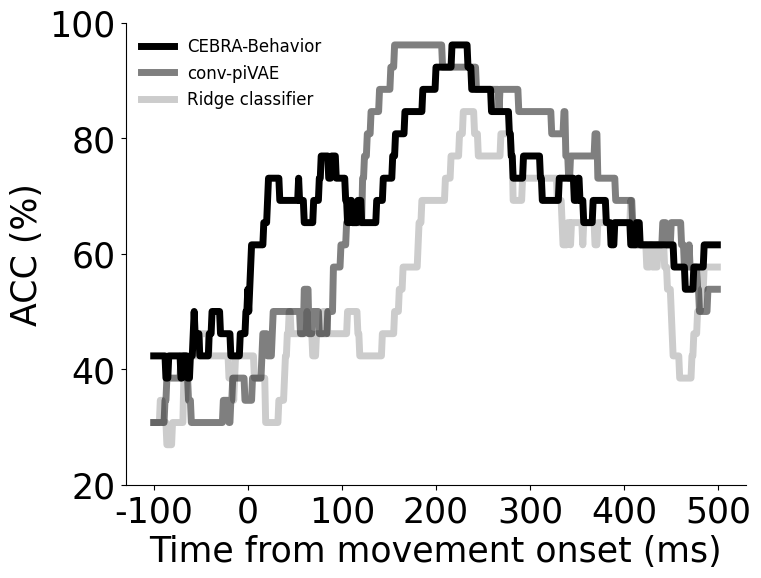
Decoding performance of on target direction using CEBRA-Behavior, conv-pi-VAE and a linear classifier.

• CEBRA-Behavior shows significantly higher decoding performance than linear classifier (one-way ANOVA, F(2,75)=3.37, p<0.05 with Post Hoc Tukey HSD p<0.05)

results = data["direction_decoding"]
cebra_acc_time = results["cebra"]
pivae_acc_time = results["pivae"]
ridge_acc_time = results["ridge"]

fig = plt.figure(figsize=(8, 6))
ax = plt.subplot(111)
ax.plot(cebra_acc_time, label="CEBRA-Behavior", color="k", lw=5)
ax.plot(pivae_acc_time, label="conv-piVAE", color="black", alpha=0.5, lw=5)
ax.plot(ridge_acc_time, label="Ridge classifier", color="k", alpha=0.2, lw=5)
# ax.plot(vel/vel.max()*100, label = 'hand speed')
ax.spines["right"].set_visible(False)
ax.spines["top"].set_visible(False)
plt.legend(frameon=False, fontsize=12)
plt.ylabel("ACC (%)", fontsize=25)
plt.yticks(np.linspace(20, 100, 5), fontsize=25)
plt.xlabel("Time from movement onset (ms)", fontsize=25)
plt.xticks(
    np.linspace(0, 600, 7, dtype=int), np.linspace(-100, 500, 7, dtype=int), fontsize=25
)
plt.show()

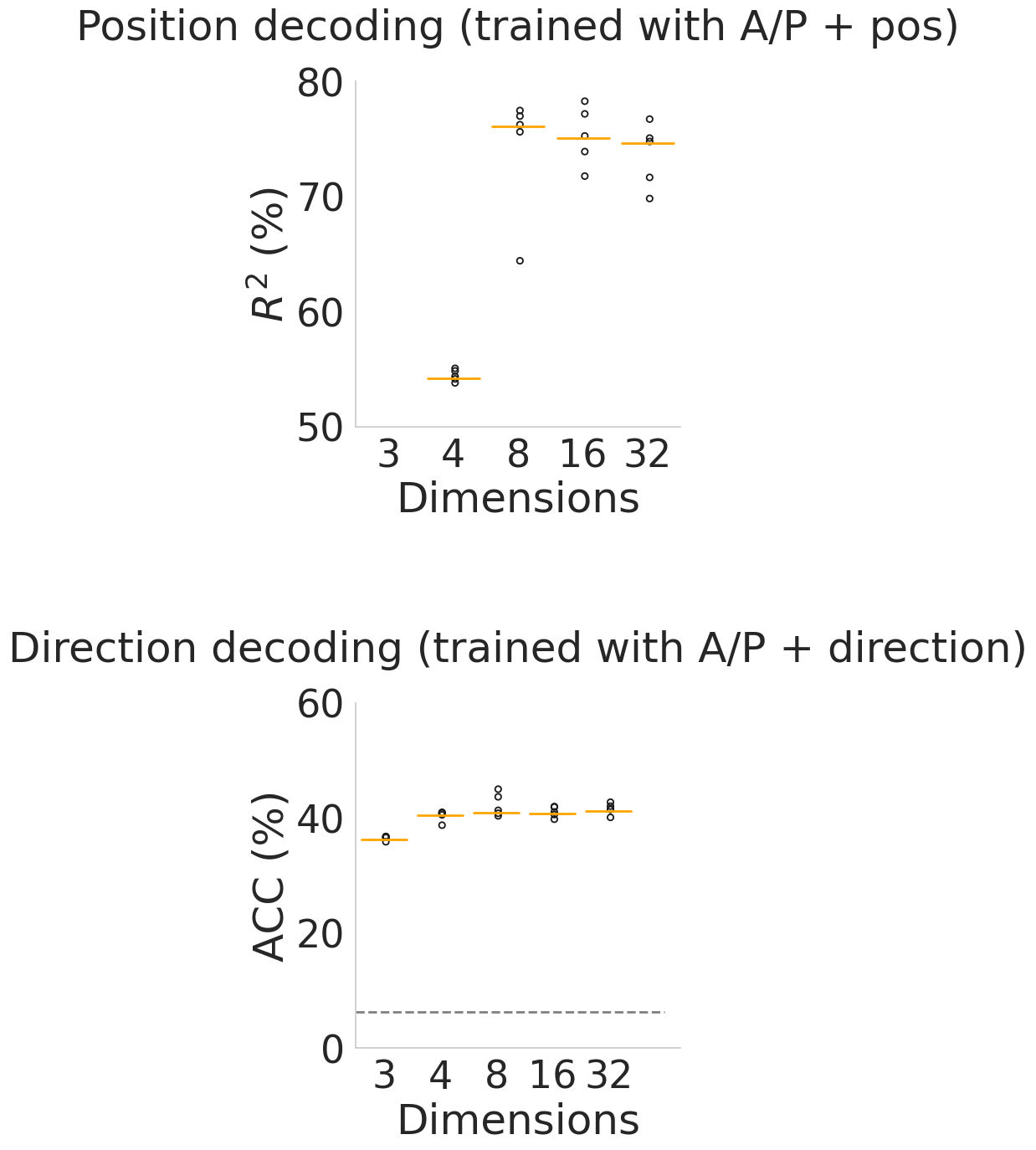
Additional decoding performance results on position and direction-trained CEBRA models with all trial types. For each case, we trained and evaluated 5 seeds represented by black dot and the orange line represents median.

## All trials
ap_position_acc = data["ap_position_dim_decoding"]
ap_direction_acc = data["ap_direction_dim_decoding"]

sns.set(font_scale=3)
sns.set_style(
    "whitegrid",
    {"axes.grid": False},
)
fig = plt.figure(figsize=(5, 15))
axs = fig.subplots(2, 1)
plt.subplots_adjust(hspace=0.8)
data_list = [ap_position_acc, ap_direction_acc]
title_list = [
    "Position decoding (trained with A/P + pos)",
    "Direction decoding (trained with A/P + direction)",
]

chance = 1 / 16
units = ["$R^2$ (%)", "ACC (%)"]
ylims = [(50, 80), (0, 60)]
for i in range(2):
    m = 0
    ax = sns.stripplot(
        data=data_list[i][["3", "4", "8", "16", "32"]],
        facecolor="none",
        color="k",
        marker="$\circ$",
        s=10,
        jitter=0,
        ax=axs[i],
    )

    sns.boxplot(
        showmeans=False,
        medianprops={"color": "orange", "ls": "-", "lw": 2},
        whiskerprops={"visible": False},
        zorder=10,
        data=data_list[i][["3", "4", "8", "16", "32"]],
        showfliers=False,
        showbox=False,
        showcaps=False,
        ax=axs[i],
    )
    if i != 0:
        axs[i].plot(
            [-0.5, 5], [chance * 100, chance * 100], lw=2, ls="dashed", c="gray"
        )

    ax.set_xlabel("Dimensions")
    ax.set_ylim(ylims[i])
    ax.set_ylabel(units[i])
    ax.set_title(title_list[i], y=1.1)
    ax.set_xticks(ticks=np.arange(5))
    ax.set_xticklabels(labels=[3, 4, 8, 16, 32])
    ax.spines["right"].set_visible(False)
    ax.spines["top"].set_visible(False)

plt.show()