You can download and run the notebook locally:

---

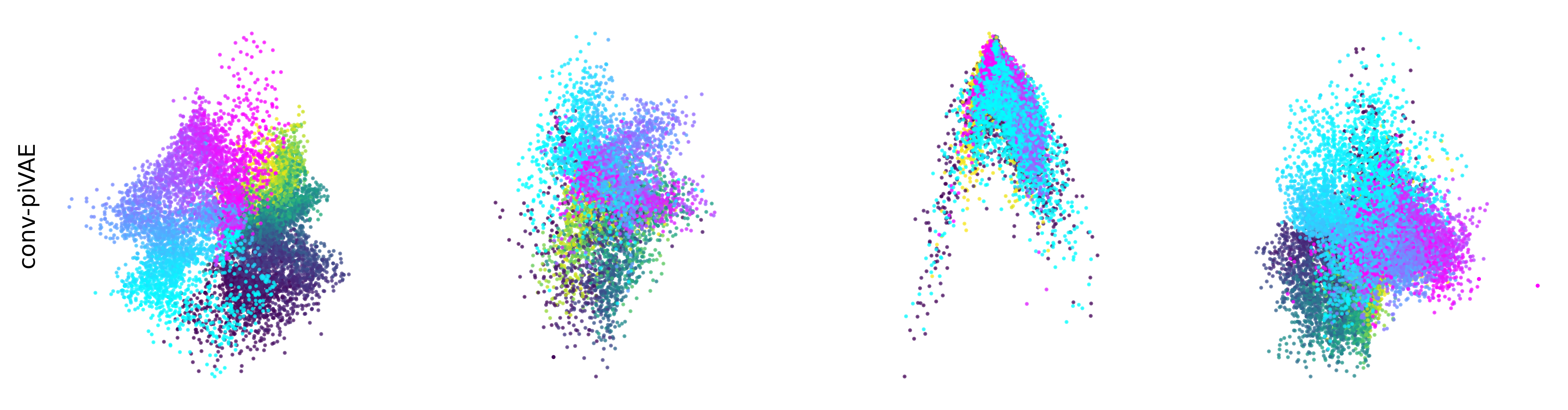
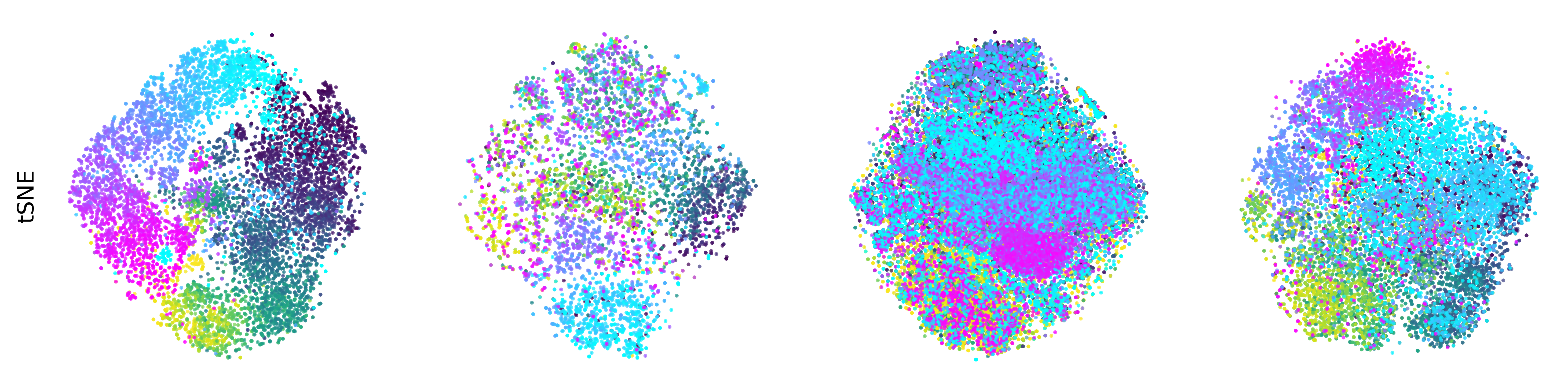
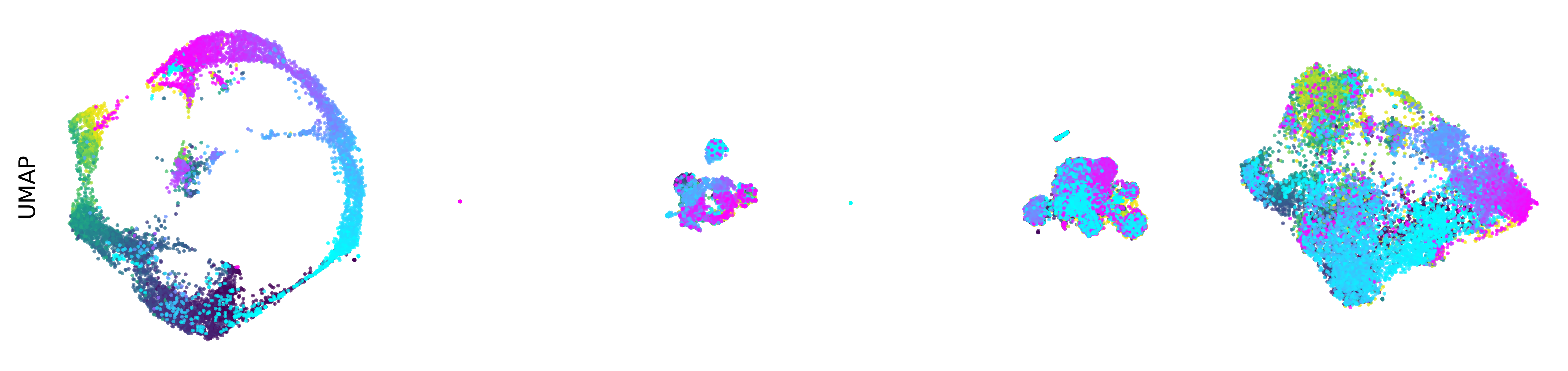
Extended Data Figure 3: CEBRA produces consistent, highly decodable embeddings

• Additional rat data shown for all algorithms we benchmarked (see Methods). CEBRA was trained with output latent on the 2-sphere (the minimum) and all other methods were obtained with a 2D latent in Euclidean space.

import pandas as pd
import matplotlib.pyplot as plt
import seaborn as sns

df = pd.concat([
  pd.read_hdf("../data/EDFigure3.h5", key="data"),
  pd.read_hdf("../data/EDFigure3_addition.h5", key="data")
], axis = 0, ignore_index = True)

def scatter(data, index, ax, s=0.01, alpha=0.5):
    mask = index[:, 1] > 0
    ax.scatter(*data[mask].T, c=index[mask, 0], s=s, cmap="viridis", alpha=alpha)
    ax.scatter(*data[~mask].T, c=index[~mask, 0], s=s, cmap="cool", alpha=alpha)


fig = plt.figure(figsize=(4 * 3, 7 * 3), dpi=600)
for i in df.index:
    ax = fig.add_subplot(7, 4, i + 1)
    scatter(df.loc[i, "emission"][:, :2], df.loc[i, "labels"], ax=ax, s=0.5, alpha=0.7)
    ax.set_yticklabels([])
    ax.set_xticklabels([])
    ax.set_xticks([])
    ax.set_yticks([])
    sns.despine(bottom=True, left=True, ax=ax)
    # first row labels
    if i // 4 == 0:
        ax.set_title(f"Rat {df.loc[i, 'animal']}", fontsize=18)
    # first column labels
    if i % 4 == 0:
        ax.set_ylabel(df.loc[i, "method"])

For a higher resolution plot, we export each row as a separate file:

def scatter(data, index, ax, s=0.01, alpha=0.5):
    mask = index[:, 1] > 0
    ax.scatter(*data[mask].T, c=index[mask, 0], s=s, cmap="viridis", alpha=alpha)
    ax.scatter(*data[~mask].T, c=index[~mask, 0], s=s, cmap="cool", alpha=alpha)

def export_highres():
  for method in df.method.unique():
      print(method)
      fig = plt.figure(figsize=(4 * 3, 1 * 3), dpi=600)
      entry = df[df.method == method].set_index("animal")
      for i, animal in enumerate(sorted(entry.index)):
          ax = fig.add_subplot(1, 4, i + 1)
          scatter(
            entry.loc[animal, "emission"][:, :2],
            entry.loc[animal, "labels"],
            ax=ax, s=0.5, alpha=0.7
          )
          ax.set_yticklabels([])
          ax.set_xticklabels([])
          ax.set_xticks([])
          ax.set_yticks([])
          ax.set_aspect("equal")
          sns.despine(bottom=True, left=True, ax=ax)
          # first row labels
          #if i // 4 == 0:
          #    ax.set_title(f"Rat {df.loc[i, 'animal']}")
          # first column labels
          if i % 4 == 0:
              ax.set_ylabel(method)
      method = method.replace('/', '-')
      plt.savefig(f'edf3_{method}.png', bbox_inches = "tight", transparent = True)
      plt.show()

export_highres()

CEBRA-Behavior

conv-piVAE w/labels

CEBRA-Time

conv-piVAE

tSNE

UMAP

autoLFADS